Geometric Transforms

DRAFT, not finalized. This chapter is new and still under review.

stough 202-

1. Homogeneous coordinates

2. The affine family

3. Composing transforms

4. Warping an image

5. Interactive: rotate and scale

6. Projective transforms

7. 🔨 Your Turn: Rectify a Photo

8. 🧠 Further Efforts

In Coordinate Operations we rotated and scaled an image with $2 \times 2$ matrices, using inverse mapping: for every pixel of the output, compute where it came from in the input, and interpolate there. That notebook ended with two loose threads.

• To rotate about the image’s center rather than its corner, we had to subtract the center, apply the matrix, and add the center back. Shifting, or translation, is not something a $2 \times 2$ matrix can do, since multiplying any matrix by the origin $\langle 0, 0 \rangle$ gives back the origin.

• Rotation, scaling and shearing all keep parallel lines parallel. But take a photo of a sheet of paper from an angle and its parallel edges converge. That warp isn’t a $2 \times 2$ matrix either.

In this notebook we tie up both threads with one idea, homogeneous coordinates, which turn translation, and then perspective, into matrix multiplication too.

Homogeneous Coordinates¶

The trick is to add a third coordinate that is always 1: the point $(x, y)$ becomes $\langle x, y, 1 \rangle$. Now a $3 \times 3$ matrix can translate:

The constant 1 in the third coordinate multiplies the last column, which adds $t_x$ and $t_y$. Our old $2 \times 2$ matrices fit in the top-left corner, with zeros beside and below and a 1 in the corner. So rotation by $\theta$, for example, becomes

One change of convention from coord_ops: there we wrote points as $(row, col)$, matching how we index an image. Here we’ll write them as $(x, y) = (col, row)$, which is what scikit-image’s transforms expect. $x$ runs to the right and $y$ runs down, because row numbers increase downward. So a positive rotation angle turns clockwise on screen.

Let’s write the basic transforms as small functions that each return a $3 \times 3$ matrix.

To see what these do, we’ll transform a shape rather than an image: the outline of a letter F, whose lack of symmetry makes it easy to tell whether it’s been rotated, flipped, or slanted. Its corners are stored as the columns of a $3 \times N$ matrix in homogeneous coordinates, so transforming every corner at once is a single matrix product, just as with coords in coord_ops.

The Affine Family¶

Any $3 \times 3$ matrix whose last row is $[0, 0, 1]$ is an affine transform:

It has six free numbers: a $2 \times 2$ linear part ($a, b, c, d$) and a translation ($t_x, t_y$). Below, the original F is dashed and the transformed F is solid.

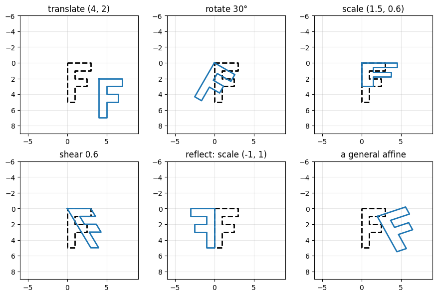
Each panel is one matrix applied to every corner of the F. A few things to notice:

• Translation slides the shape without turning or resizing it.

• Rotation turns it about the origin, the top-left corner of the grid at $(0, 0)$, not about the F’s own center. Since $y$ points down, a positive angle turns clockwise.

• Scaling by different amounts in $x$ and $y$ squashes the F. A negative scale flips it: that’s a reflection.

• Shear slides each point sideways in proportion to its height, the way a deck of cards slants when you push it sideways.

• The general affine does all of these at once.

And here’s what all affine transforms have in common: straight lines stay straight, and parallel lines stay parallel. The F’s two arms stay parallel to each other in every panel, even when they’re no longer horizontal. Lengths and angles can change, but parallelism can’t. Keep that in mind for later.

Composing Transforms¶

The payoff of making everything a matrix is that a sequence of transforms is just a product of matrices. If we first apply $\mathbf{A}$ and then $\mathbf{B}$ to a point $\mathbf{p}$, we get $\mathbf{B}(\mathbf{A}\mathbf{p}) = (\mathbf{B}\mathbf{A})\mathbf{p}$. So the single matrix $\mathbf{B}\mathbf{A}$ does both. Note the order: the transform applied first is written on the right.

Matrix multiplication isn’t commutative, and neither are transforms. Rotating and then translating is not the same as translating and then rotating:

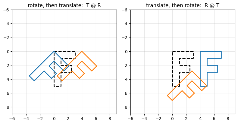
In each panel the dashed F is the original, blue is after the first step, and orange is after both. On the left, the F rotates about the origin and then slides 4 units to the right. On the right, it first slides right, and then the rotation swings it, along with everything else, about the origin, so it ends up below and to the left of the blue F: rotated by the same angle, but in a different place.

This also explains the rotation about the center from coord_ops. To rotate about a point $\mathbf{c}$: translate $\mathbf{c}$ to the origin, rotate, and translate back. As one matrix, that’s

read right to left. Let’s check with the center of the F.

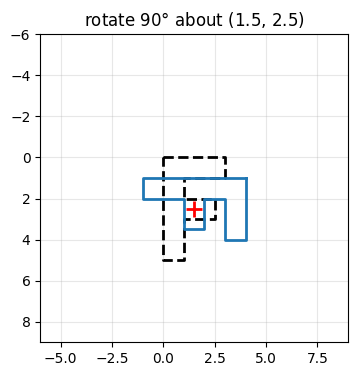
Three matrices multiplied into one. The result is still affine (its last row is still $[0, 0, 1]$), and the F turns in place about the red cross. Look at the printed matrix: its top-left $2 \times 2$ block is just the $90°$ rotation, and the last column is the translation that keeps the center fixed. However long a chain of affine transforms gets, it always collapses to a single affine matrix, so warping an image by the whole chain costs no more than warping by one transform.

Warping an Image¶

Now let’s apply transforms to an image. We could reuse the inverse-mapping code from coord_ops, but scikit-image’s warp does exactly the same job: for every output pixel, it asks a map where that pixel comes from in the input, and interpolates there. AffineTransform wraps a $3 \times 3$ matrix as a map.

There’s one catch, and it trips up everyone at least once. Because warp works by inverse mapping, the map you give it must go from output coordinates back to input coordinates. That’s the inverse of the transform you want to see. Every transform object has an .inverse for exactly this purpose.

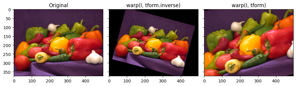
M was meant to shrink the peppers to 80% and turn them $15°$ clockwise about the center. With tform.inverse, that’s what we get. With tform itself, warp applies the inverse of what we meant: the image grows by $1/0.8 = 1.25$ and turns counterclockwise. When a warp comes out backwards, this is the first thing to check.

Output pixels whose source lands outside the input are filled with 0 (black), just like our valid mask in coord_ops. And warp takes the same interpolation order as map_coordinates and rescale: 0 for nearest neighbor, 1 for bilinear (the default), 3 for bicubic.

Interactive: Rotate and Scale¶

Here are the same transforms with sliders. Each update builds one composite matrix, rotation and scaling about the image center, and calls warp once.

Projective Transforms¶

Affine transforms keep parallel lines parallel. A camera doesn’t. When you photograph a flat surface from an angle, such as a page, a sign, or a tiled floor, the parallel edges that recede from you converge toward a vanishing point. Here’s scikit-image’s text sample image, a photo of handwriting on a board, taken at an angle.

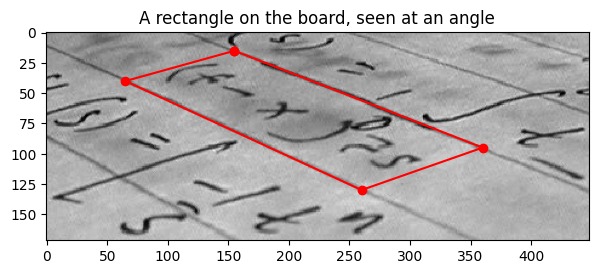
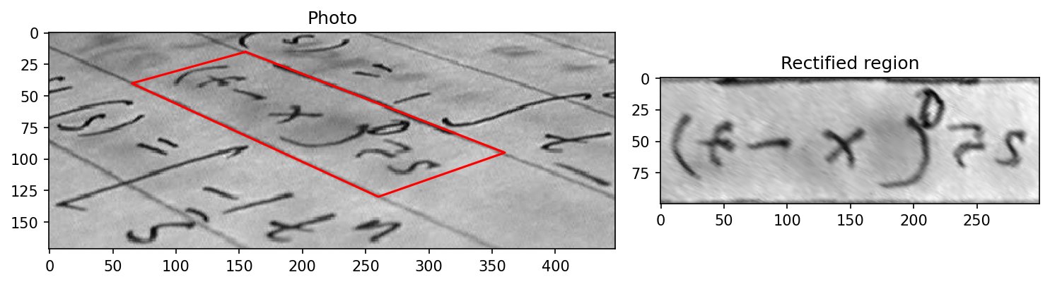
The red outline marks a region that is a rectangle on the board itself, but in the photo it’s a slanted quadrilateral, and its opposite sides aren’t parallel. No affine transform can turn it back into a rectangle.

The fix is to free up the last row of the matrix. A projective transform, or homography, is a general $3 \times 3$ matrix

With $g$ and $h$ nonzero, the third coordinate $w$ is no longer 1, so we divide by it to get back to a point in the plane. That division makes points farther along the $(g, h)$ direction shrink toward each other, which is exactly the perspective effect. Straight lines still map to straight lines, but parallel lines can now meet. The bottom-right entry is fixed at 1 because scaling the whole matrix doesn’t change $u/w$ and $v/w$, which leaves 8 free numbers.

Estimating a homography from four points. Where does the matrix come from? If we know where four points go, we know it. Each point pair $(x, y) \to (x', y')$ gives two equations. Multiplying out the denominator of the first,

which is linear in the 8 unknowns, and similarly for $y'$. Four point pairs give 8 linear equations in 8 unknowns: a system we can solve with np.linalg.solve. Let’s map our four corners to the corners of a $300 \times 100$ rectangle.

Our 8-by-8 solve and scikit-image agree. Notice that $g$ and $h$, the first two entries of the bottom row, are small but not zero: that’s the perspective.

Now we rectify. The homography maps the photo to the rectangle, so, just as with the affine warp, we hand warp its inverse, and ask for an output the size of the rectangle.

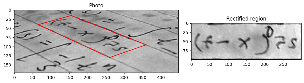
The slanted region now reads as if we were looking straight at the board: the handwritten expression runs straight across, upright and evenly sized. This is how document-scanning apps flatten a photo of a page, and how sports broadcasts paint lines onto a field.

Two caveats. First, the photo only tells us where the corners are, not the region’s true shape, so we had to choose the $300 \times 100$ output. If we pick the wrong aspect ratio, the writing comes out stretched. Second, in a strongly slanted photo the far side of a surface covers fewer pixels than the near side, so the far end of the rectified image comes out blurrier: it’s been interpolated from less data. Rectifying can’t recover detail the camera never recorded.

🔨 Your Turn: Rectify a Photo¶

Task: Take a photo of something flat and rectangular, at an angle: a page, a poster, a whiteboard, a laptop screen, or the face of a building. Rectify it so that you seem to be looking straight at it. Show the photo with the four corners marked, next to the rectified result.

Guidance:

• Load your photo with plt.imread and check it with arr_info. Shrink a phone photo first (e.g. with skimage.transform.rescale), since a 12-megapixel warp is slow; remember to find the corners on the shrunken image.

• To find the corner coordinates, display the image in an interactive (%matplotlib widget) figure and hover over each corner: the $(x, y)$ position appears in the figure’s toolbar. Keep the corners in the same order (say clockwise from the top left) in both point lists.

• You need to choose the output rectangle’s size. If you know the object’s real shape (a letter-size page is $8.5 \times 11$ inches), use its aspect ratio. If you don’t, how could you estimate it from the photo?

• If the result comes out mirrored, rotated, or as a strange sliver, check the order of your corners and whether you passed warp the transform or its inverse.

• For a color photo, warp handles all three channels at once.

🧠 Further Efforts¶

1. Which transforms commute? We saw that rotation and translation don’t commute. Which pairs of the basic transforms do: two rotations? Two translations? A rotation and a uniform scaling? A rotation and a non-uniform scaling? Predict each one first, and then check by comparing the matrix products.
   Guidance: np.allclose(A @ B, B @ A) checks it numerically. For the ones that don’t commute, draw both orders with show_shapes to see the difference.

2. Affine from three points. A homography needs four point pairs to pin down. How many does an affine transform need, and why? Write affine_from_3_points(src, dst) in the style of homography_from_4_points, and check it against AffineTransform().estimate.
   Guidance: Count the unknowns and the equations each point pair provides. What happens when your three points lie on a line?

3. Image registration. Warp the peppers image with an affine transform that you keep secret (put it in a variable you don’t look at). Then recover the transform by finding three or more matching points in the two images, estimate it, and undo the warp. How close do you get back to the original?
   Guidance: Choose points that are easy to locate precisely in both images, such as the tips of stems. With more than three pairs, estimate finds the least-squares fit, which averages out your clicking errors. Measure the result with the mean absolute difference from the original, ignoring the black border.