Spatial Operations - imageprocessing-awesome

stough 202-

Predictive Coding from spatial operations perspective
Unsharp Masking
Gradient Maps
Summary
🧠 Further Efforts

To this point we have generally thought of images as collections of independent pixels, organized in a grid for sure but not really thought of as a connected collection. We have heavily considered the histograms of images for use in contrast enhancement and compression, where histogramming completely destroys the spatial relationships that these pixels have with one another. In considering entropy in fact, we modeled our image as a sequence of independent and identically distributed (iid) symbols sampled from the histogram (probability distribution).

We did hint at the importance of spatial coherence, which is exactly the way in which images are not iid sequences. We saw that predictive coding, using neighbors of a pixel to predict that pixel and then encoding only the error of prediction, leads to much more highly compressible signals than the images themselves. Were pixels iid, then such an encoding would be of no benefit. If our power transform is an example of a single-pixel operation (or point transform), then predictive coding is an example of a spatial or neighborhood operation.

Spatial operations are operations that we apply to the pixels of an image that take into account the neighborhood of a pixel. Linear versions of such operations are also called spatial filters. We’re basically looking at the neighborhood of a pixel and computing a linear combination of the values/intensities in that neighborhood.

Here we’re going to look at some spatial operations using scipy.ndimage.correlate.

Imports¶

Bringing in scipy.ndimage.correlate and convolve.

%matplotlib inline
import matplotlib.pyplot as plt
import numpy as np

# For spatial filtering/operations
from scipy.ndimage import (correlate,
                           convolve)

# For importing from alternative directory sources
import sys  
sys.path.insert(0, '../dip_utils')

from matrix_utils import (arr_info,
                          make_linmap)
from vis_utils import (vis_rgb_cube,
                       vis_hists,
                       vis_pair)

Review Predictive Coding¶

In predictive coding we predicted each pixel by its left neighbor and kept only the difference. Instead of directly using np.diff, we can use correlate: slide the tiny filter $h = [-1, 1]$ across the image, and at every position compute the sum of the products of the filter with the pixels under it. That’s $J(r,c) - J(r,c-1)$ , the prediction error.

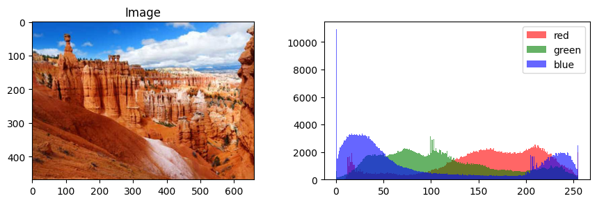
I = plt.imread('../dip_pics/canyon.jpg')
vis_hists(I)
print(arr_info(I))

((469, 660, 3), dtype('uint8'), np.uint8(0), np.uint8(255))

J = I[...,0]
vis_hists(J)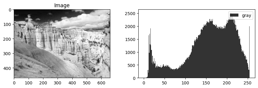

h = np.array([-1, 1], ndmin=2).astype('int16')

array([[-1, 1]], dtype=int16)

arr_info(h)

((1, 2), dtype('int16'), np.int16(-1), np.int16(1))

Note the int16 type, for both the filter and (below) the image: the difference of two uint8 values can be negative, and as unsigned 8-bit integers those would wrap around to large positive numbers. ndmin=2 makes h a $1 \times 2$ 2D array, so correlate treats it as a horizontal filter on our 2D image.

Jf = correlate(J.astype('int16'), h, mode='constant', cval=0)
arr_info(Jf)

((469, 660), dtype('int16'), np.int16(-113), np.int16(238))

vis_hists(Jf)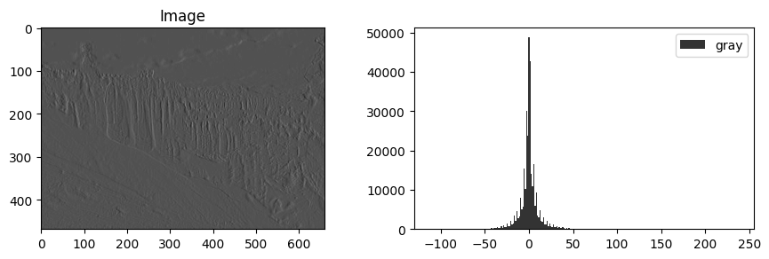

Unsharp Masking¶

Above we saw how to use a spatial filter to get at local pixel differences. Here we’ll use a blur to actually sharpen the edges in an image. In the below, we basically recalculate every pixel to actually be the average of its neighborhood, here just a 5x5 neighborhood.

h = np.ones((5,5))/25.0
h

array([[0.04, 0.04, 0.04, 0.04, 0.04],
       [0.04, 0.04, 0.04, 0.04, 0.04],
       [0.04, 0.04, 0.04, 0.04, 0.04],
       [0.04, 0.04, 0.04, 0.04, 0.04],
       [0.04, 0.04, 0.04, 0.04, 0.04]])

Jf = correlate(J.astype('float'), h, mode='constant', cval=0)

vis_pair(J, Jf, cmap='gray', second_title="Blurred")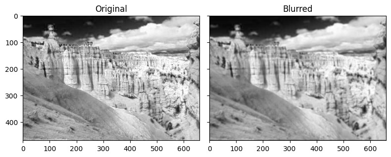

arr_info(Jf)

((469, 660), dtype('float64'), np.float64(5.0), np.float64(254.63999999999996))

arr_info(J)

((469, 660), dtype('uint8'), np.uint8(0), np.uint8(255))

D = J - Jf
vis_hists(D)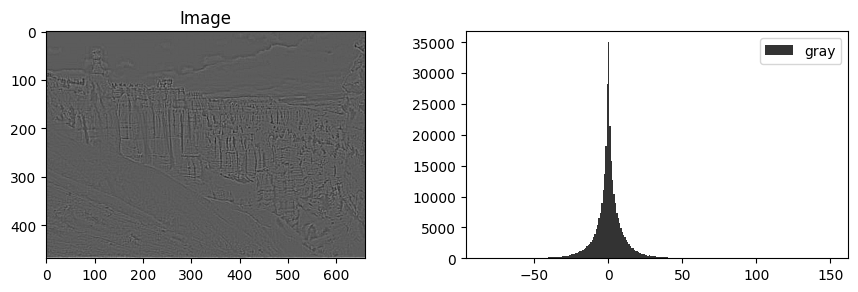

vis_pair(J, D, cmap='gray', second_title='Original - Blurred')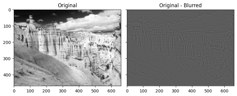

Jsharp = J + 2*D 
# vis_pair(J, Jsharp, cmap='gray') # results in less contrast due to out-of-range pixels messing up display.
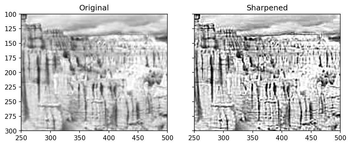
vis_pair(J, np.clip(Jsharp,0,255), cmap='gray', second_title="Sharpened")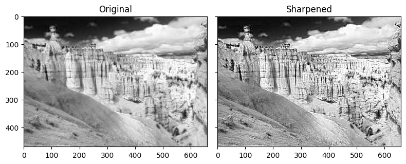

arr_info(Jsharp)

((469, 660),
 dtype('float64'),
 np.float64(-145.76000000000002),
 np.float64(531.72))

plt.figure(figsize=(5,3))
plt.plot(J[193, 250:270], label='original')
plt.plot(np.clip(Jsharp,0,255)[193, 250:270], label='sharpened')
plt.xlabel('column (offset from 250)')
plt.ylabel('intensity, row 193')
plt.legend()
plt.tight_layout()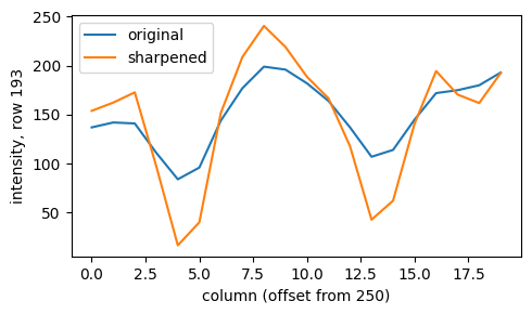

Putting the steps together, unsharp masking computes

J_{sharp} = J + k\,(J - \bar{J})

where $\bar{J}$ is the blurred image and $k$ (here 2) sets the strength. The difference $J - \bar{J}$ is the “detail” that blurring removed: positive on the bright side of an edge, negative on the dark side, and near zero in smooth regions. Adding back an amplified copy pushes the bright side brighter and the dark side darker.

The profile plot along one row shows it directly: the sharpened curve exaggerates every peak and valley of the original. At a real edge this overshoot is what our eyes read as crispness, but push $k$ too far and it becomes a visible bright/dark halo along edges, a telltale sign of an over-sharpened photo. (The name comes from the darkroom, where the blurred, “unsharp” negative was used as a mask.) We’ll see this same idea from the filter’s point of view in high-pass filtering, and from the frequency point of view in Fourier sharpening.

Gradient Maps¶

An alternative filter design can give us locally computed vertical and horizontal edginess if you will. These first order derivative images in $x,y$ can allow us to compute the gradient map of an image. Basically the edginess of every pixel.

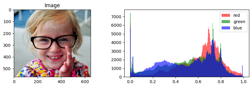
I = plt.imread('../dip_pics/girl_with_glasses.png')
vis_hists(I)
print(arr_info(I))

((570, 649, 4), dtype('float32'), np.float32(0.0), np.float32(1.0))

h = np.ones((5,5))/25.0
h

array([[0.04, 0.04, 0.04, 0.04, 0.04],
       [0.04, 0.04, 0.04, 0.04, 0.04],
       [0.04, 0.04, 0.04, 0.04, 0.04],
       [0.04, 0.04, 0.04, 0.04, 0.04],
       [0.04, 0.04, 0.04, 0.04, 0.04]])

h = np.array([[1, 0, -1],[2, 0, -2],[1, 0, -1]])

array([[ 1,  0, -1],
       [ 2,  0, -2],
       [ 1,  0, -1]])

This filter we’ve designed above responds to vertical edges; that is, to get a large magnitude response from correlation with a 3x3 image neighborhood, we would need the left side of this tiny neighborhood to look brighter than the right (or darker for a large negative response). This is the famous Sobel operator, which you can read more about here and here.

plt.figure()
plt.imshow(h, cmap='gray')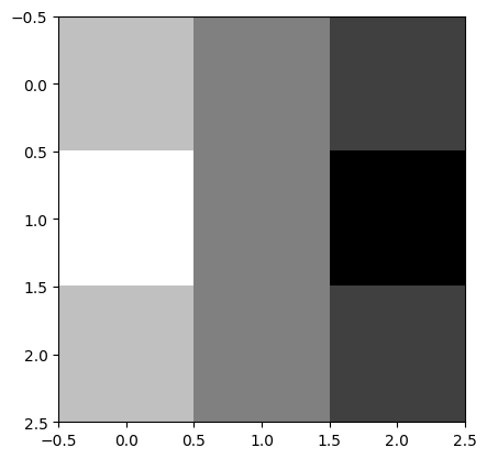

Gx = correlate(I[...,0], h, mode='nearest')

vis_pair(I, Gx, cmap='gray', second_title="GX")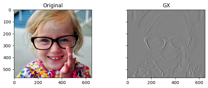

Gy = correlate(I[...,0], h.transpose(), mode='nearest')

vis_pair(Gx, Gy, cmap='gray', first_title='Gx', second_title='Gy')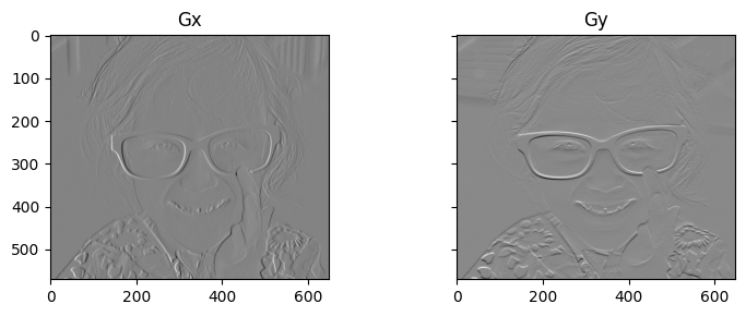

The above are the first order derivatives in $x$ and $y$ for the original image when thought of as a height map, and using the Sobel operators to compute local difference.

The gradient magnitude (how steep the height map is) is then the square root of the sum of the squared derivatives:

|\nabla I| = \sqrt{G_x^2 + G_y^2}

Thinking of the image as a height map, $G_x$ and $G_y$ are the slopes in the two directions, and $|\nabla I|$ is the steepness of the terrain regardless of direction. Edges are the cliffs.

G = np.sqrt(Gx**2 + Gy**2)
# G = Gx**2 + Gy**2

arr_info(G)

((570, 649), dtype('float32'), np.float32(0.0), np.float32(3.4203362))

vis_pair(I, G.max() - G, cmap='gray', second_title='Grad Mag')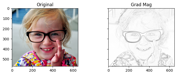

Laplacian¶

The gradient uses first derivatives; the Laplacian is a sum of second derivatives:

\nabla^2 I = \frac{\partial^2 I}{\partial x^2} + \frac{\partial^2 I}{\partial y^2}

A second derivative measures curvature: how much a pixel differs from the average of its neighbors. The filter below does exactly that: 8 times the center minus the sum of the 8 neighbors. It is zero in flat regions and on constant slopes, and responds strongly on either side of an edge (with opposite signs). It has no direction, so one filter catches edges at every orientation. Because it amplifies pixel-to-pixel differences, though, it is also very sensitive to noise.

h = np.array([[-1, -1, -1],[-1, 8, -1],[-1, -1, -1]])

array([[-1, -1, -1],
       [-1,  8, -1],
       [-1, -1, -1]])

J = correlate(I[...,0], h, mode='nearest')
arr_info(J)

((570, 649), dtype('float32'), np.float32(-1.6980393), np.float32(2.0039215))

J = np.abs(J)
J = J/J.max()
arr_info(J)

((570, 649), dtype('float32'), np.float32(0.0), np.float32(1.0))

vis_pair(I, 1 - np.log2(J+1),  cmap='gray')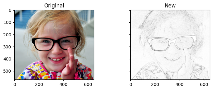

Summary¶

In this notebook we moved from point operations, which treat every pixel independently, to spatial operations, which compute each output pixel from a neighborhood of input pixels. All of the ones we saw are linear spatial filters: correlate slides a small kernel of weights over the image and computes a weighted sum at every position.

Predictive coding is a filter: the left-neighbor difference kernel $[-1, 1]$ . Its output is small almost everywhere because neighboring pixels are similar.
Unsharp masking blurs the image with a box kernel, subtracts the blur to isolate the fine detail, and adds a multiple of that detail back to sharpen.
Gradient maps: the Sobel kernels estimate the derivatives $G_x$ and $G_y$ , and the gradient magnitude $\sqrt{G_x^2 + G_y^2}$ measures how steeply the intensity changes at each pixel, regardless of direction.
The Laplacian is a second-derivative kernel. It measures how much each pixel differs from its neighbors, in every direction at once.

Next, we’ll look more closely at the kernels themselves, as 3D height maps, and then at smoothing, sharpening, and edge detection in turn.

🧠 Further Efforts¶

Diagonal edges. Our Sobel kernels respond to vertical and horizontal edges. Design kernels in the same spirit that respond to edges at $45°$ and $135°$ , and show their responses for the image. Which features of the image respond most strongly to each?
Guidance: Look at the pattern of weights in h: a column of positive weights, a column of zeros, a column of negatives. Rotate that pattern, rather than the numbers’ positions blindly, and check that the weights still sum to zero. Test your kernels on a synthetic image of a diagonal edge before using the photo.
Unsharp masking at different scales. Repeat the unsharp masking with box blurs of size $3 \times 3$ , $9 \times 9$ and $21 \times 21$ . What gets sharpened in each case?
Guidance: Keep $k$ fixed while you change the blur size. A small blur isolates fine texture; think about what the difference $J - \bar{J}$ contains when the blur is large. Large boxes are faster with uniform_filter than with correlate.
Different kinds of images. Apply unsharp masking and the gradient magnitude to a scanned text document, a medical image such as ../dip_pics/chestCT.jpg, and a natural scene. Which operations are most helpful for which kind of image?
Guidance: For each one, decide first what you’d want to enhance (strokes of text, organ boundaries, texture), and then judge the operation by that goal.