Exploring Spatial Filters, as 3D height maps

stough 202-

In spatial_ops we saw how we could correlate or filter an image with a particular mask or filter, in order to compute something about the local neighborhood around every pixel in an image. We saw a blurring filter, vertical and horizontal edge detecting filters, and the LaPlacian. Here we’ll take a closer look at these filters. Viewing a kernel as a little height map makes it easier to see what it does: where its weights are positive or negative, and how quickly they fall off.

%matplotlib inline
import matplotlib.pyplot as plt
from matplotlib import cm
import numpy as np

# For spatial filtering/operations
from scipy.ndimage import (correlate,
                           convolve)
from scipy.stats import (norm, 
                         entropy)

# For importing from alternative directory sources
import sys  
sys.path.insert(0, '../dip_utils')

from matrix_utils import (arr_info,
                          make_linmap)
from vis_utils import (vis_rgb_cube,
                       vis_hists,
                       vis_pair)

Blurring¶

Though the filters themselves might be small (3x3, 11x11) relative to the size of the image, we’re going to upsample them here, so we can look at the ideal versions as 3D heightmaps.

When blurring, we can use either a flat filter, giving equal weight to every pixel in the neighborhood, or we can do a smoother Gaussian kind of blur, where we give more weight to pixels closer to the center.

x = np.arange(-2.5,2.5,.1)
y_flat = .2*np.ones_like(x) # times .2 just for scaling of the plot
y_gaussian = norm.pdf(x)

y_gaussian.sum(), y_flat.sum()

(np.float64(9.87507674347893), np.float64(9.999999999999998))

Both sums are about 10, and I chose the flat filter’s height so they’d match. A blurring kernel’s weights should sum to the same constant (really 1, after normalizing), so that blurring changes how the neighborhood is averaged but not the overall brightness. That’s the same normalization we used in the low-pass demo.

plt.figure(figsize=(4,3))
plt.plot(x, np.transpose([y_flat, y_gaussian]));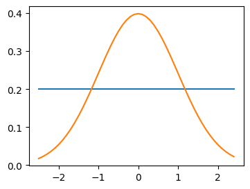

View in 3D¶

X2d, Y2d = np.meshgrid(x, x, indexing='ij')

fig = plt.figure(figsize=(4,4))
ax = fig.add_subplot(111, projection='3d')

ax.plot_surface(X2d, Y2d, np.outer(y_gaussian, y_gaussian), cmap=cm.coolwarm);
plt.tight_layout()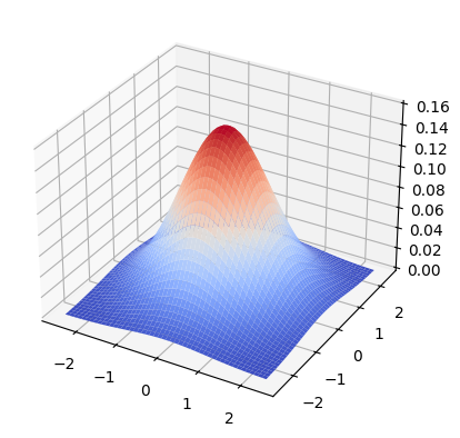

The 2D Gaussian kernel is the outer product of the 1D Gaussian with itself, a smooth, round hill. Correlating with it replaces each pixel with a weighted average that trusts the center most and fades out evenly in every direction.

Edge Detecting Filters¶

We saw the simple Sobel filters, like:

\mathbf{h_{Sobel}} = \begin{vmatrix} 1 & 0 & -1 \\ 2 & 0 & -2 \\ 1 & 0 & -1 \end{vmatrix}

This is really just an approximation of the derivative of a Gaussian in one direction. We can plot this in 3D in ideal form by taking the local difference in one of the dimensions. Again, you can read more about Sobel here and here.

plt.figure(figsize=(4,3))
plt.plot(x, np.transpose([y_gaussian, 10*np.gradient(y_gaussian)])); # times 10 just for scaling.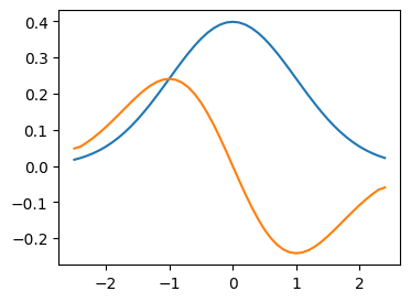

fig = plt.figure(figsize=(4,4))
ax = fig.add_subplot(111, projection='3d')

ax.plot_surface(X2d, Y2d, np.outer(np.gradient(y_gaussian), y_gaussian), cmap=cm.coolwarm);
plt.tight_layout()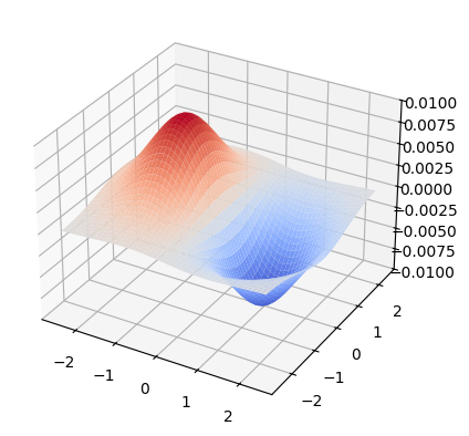

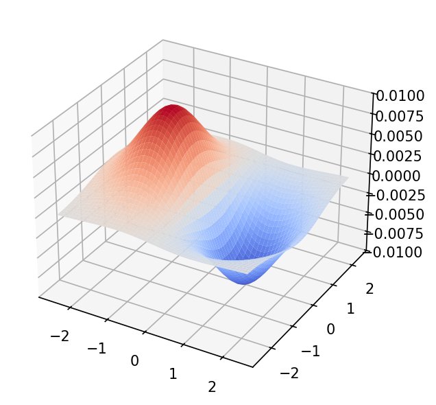
This derivative-of-Gaussian kernel is the smooth version of Sobel: a positive lobe on one side, a negative lobe on the other, and zero along the middle. Correlated with an image, it responds strongly where intensity changes along the first axis, and gives near zero in flat areas or for edges running the other way. Along the second axis it’s still a Gaussian, so it also blurs in that direction, which makes it less sensitive to noise than a bare difference. Sobel’s $[1, 2, 1]$ weighting across its three rows is a tiny approximation of exactly that blur.

Second Derivatives and the Laplacian¶

Whereas the above is a uni-directional edge detecting filter, we also saw the laplacian filter:

\mathbf{h_{Laplace}} = \begin{vmatrix} -1 & -1 & -1 \\ -1 & 8 & -1 \\ -1 & -1 & -1 \end{vmatrix}

Turns out, this is just a 3x3 version of the (negated) second derivative, summed over both directions. We’ll negate our ideal versions too, so the peak is high instead of low. First, the second derivative of a Gaussian in one direction:

plt.figure(figsize=(4,3))
plt.plot(x, np.transpose([np.gradient(y_gaussian), 
                          10*np.gradient(np.gradient(y_gaussian))])); # times 10 for scaling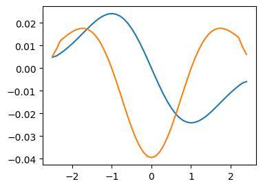

fig = plt.figure(figsize=(4,4))
ax = fig.add_subplot(111, projection='3d')

ax.plot_surface(X2d, Y2d, np.outer(-np.gradient(np.gradient(y_gaussian)), 
                                   y_gaussian), 
                cmap=cm.coolwarm);
plt.tight_layout()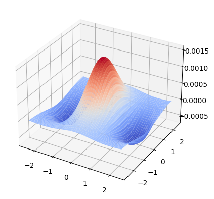

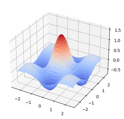
The Laplacian sums the second derivatives in the two directions, $\nabla^2 = \frac{\partial^2}{\partial x^2} + \frac{\partial^2}{\partial y^2}$ . For our separable Gaussian $G(x,y) = g(x)\,g(y)$ , that’s $g''(x)\,g(y) + g(x)\,g''(y)$ . Negated, this is the famous “Mexican hat”, the Laplacian of Gaussian (LoG): a positive peak surrounded by a negative ring, the same in every direction. Our $3 \times 3$ kernel, 8 surrounded by -1s, is a tiny version of it.

g2 = np.gradient(np.gradient(y_gaussian))
LoG = -(np.outer(g2, y_gaussian) + np.outer(y_gaussian, g2))

fig = plt.figure(figsize=(4,4))
ax = fig.add_subplot(111, projection='3d')

ax.plot_surface(X2d, Y2d, LoG, cmap=cm.coolwarm);
plt.tight_layout()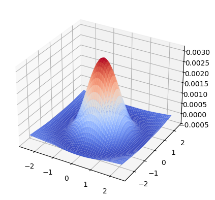

For comparison, the next plot is the product of the two second derivatives, $g''(x)\,g''(y)$ , which is a fourth-order derivative $\frac{\partial^4 G}{\partial x^2 \partial y^2}$ rather than the Laplacian. Its alternating lobes respond to checkerboard-like patterns rather than to edges in general. Compare its shape to the rotationally symmetric LoG above.

fig = plt.figure(figsize=(4,4))
ax = fig.add_subplot(111, projection='3d')

ax.plot_surface(X2d, Y2d, np.outer(np.gradient(np.gradient(y_gaussian)), 
                                   np.gradient(np.gradient(y_gaussian))), 
                cmap=cm.coolwarm);
plt.tight_layout()