Exploring spatial filtering, high pass - imageprocessing-awesome

Preview: Exploring spatial filtering, high pass

Joshua Stough DIP 3.6 on high-pass. See correlate

Here we’re going to look at the high-pass spatial filter, which derives from the local second derivative. See these cool visualizations of the Gaussian and its derivatives, and read here.

%matplotlib inline
import matplotlib.pyplot as plt
import numpy as np

# For spatial filtering/operations
from scipy.ndimage import (correlate,
                           convolve)

# For importing from alternative directory sources
import sys  
sys.path.insert(0, '../dip_utils')

from matrix_utils import (arr_info,
                          make_linmap)
from vis_utils import (vis_rgb_cube,
                       vis_hists,
                       vis_pair)

plt.style.use('dark_background')

I = plt.imread('../dip_pics/cat_small.png').astype('float')
arr_info(I)

((512, 512, 4), dtype('float64'), np.float64(0.0), np.float64(1.0))

vis_hists(I)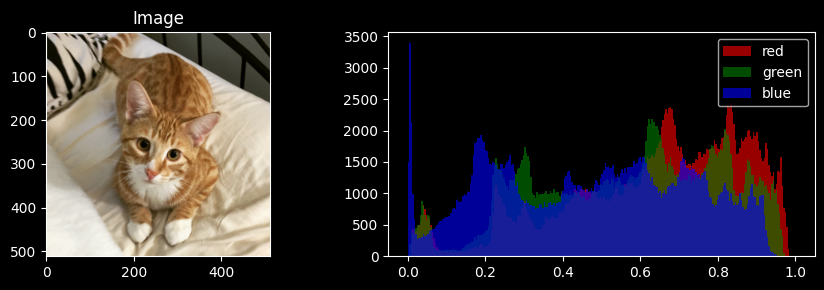

# The image includes an alpha channel that we're not going to need.
I = I[...,:3].copy()
arr_info(I)

((512, 512, 3),
 dtype('float64'),
 np.float64(0.0),
 np.float64(0.9882352948188782))

High-pass filtering, involves computing a pixel’s difference from its neighborhood¶

laplace_h = -1*np.ones((3,3))
laplace_h[1,1] = 8
laplace_h

array([[-1., -1., -1.],
       [-1.,  8., -1.],
       [-1., -1., -1.]])

Where does this kernel come from? In 1D, the second derivative of a sampled signal is approximated by the difference of differences:

f''(x) \approx [f(x+1) - f(x)] - [f(x) - f(x-1)] = f(x+1) - 2f(x) + f(x-1)

which is correlation with $[1, -2, 1]$ . Adding the second differences in $x$ and $y$ gives the 4-neighbor Laplacian kernel with -4 at the center and 1 at the four direct neighbors, and including the diagonals gives the 8-neighbor version. Our kernel is the negative of that 8-neighbor Laplacian (8 at the center, -1 around it); the sign convention is chosen so that we can simply add it to sharpen.

Two properties to notice:

The weights sum to zero, so in any flat region the response is exactly 0. Unlike the blurring kernels, this filter throws away the average brightness and keeps only the differences. It’s a high-pass filter.
Since $8 = 9 - 1$ , this kernel is exactly $9 \times$ (the pixel minus the average of its $3 \times 3$ neighborhood). So it measures how much each pixel stands out from its surroundings.

I_laplace = np.stack([correlate(I[...,i], laplace_h) for i in range(3)], axis=-1)

vis_pair(I, I_laplace)

Clipping input data to the valid range for imshow with RGB data ([0..1] for floats or [0..255] for integers). Got range [-1.5254902429878712..4.552941180765629].

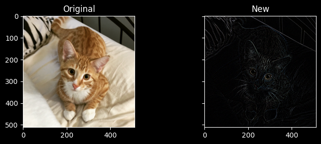
The filtered image is mostly black: about two-thirds of its values are within $\pm 0.05$ of zero, the flat regions. What’s left are outlines: the cat’s fur, whiskers and eyes, and the stripes of the pillow. (I_laplace actually ranges from about -1.5 to 4.3; imshow clips the display to $[0,1]$ , so we’re only seeing its positive part here.)

Some fraction of the LaPlace can simply be added to the original image¶

to enhance edges.

def addLap(frac):
    global I, I_laplace
    temp = I + frac*I_laplace
    return np.clip(temp, 0,1)

I_halfL = addLap(.5)
I_1L = addLap(1)
I_2L = addLap(2)

# Vis all three.
f, ax = plt.subplots(1,4, figsize=(10,3), sharex=True, sharey=True)
ax[0].imshow(I)
ax[0].set_title('Original')

ax[1].imshow(I_halfL)
ax[1].set_title('+.5*LaPlace')

ax[2].imshow(I_1L)
ax[2].set_title('+1*LaPlace')

ax[3].imshow(I_2L)
ax[3].set_title('+2*LaPlace')

plt.suptitle('Adding Edginess to Cat');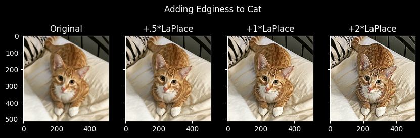

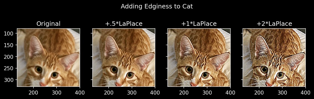
Adding the Laplacian back to the image, $I + \alpha L$ , boosts each pixel by how much it differs from its neighbors: pixels brighter than their surroundings get brighter, darker ones get darker. That makes edges crisper. With larger $\alpha$ the image starts to look harsh and noisy, since every bit of fine texture and noise is amplified along with the edges.

If this sounds familiar, it should. Since $L = 9(I - \bar{I})$ where $\bar{I}$ is the $3 \times 3$ average, adding $\alpha L$ is exactly the unsharp masking we did earlier with a $3 \times 3$ blur and $k = 9\alpha$ . Sharpening by “adding the Laplacian” and sharpening by “subtracting a blur” are the same idea.

Interactive Visualization¶

See jupyter-matplotlib

from ipywidgets import VBox, FloatSlider

pass  # (static) plt.ioff()
plt.clf()

slider = FloatSlider(
    orientation='horizontal',
    value=1.0,
    min=0.00,
    max=5.0,
    description='How much Laplace to add'
)

fig_args = {'num':' ', 'frameon':True, 'sharex':True, 'sharey':True}
fig, ax = plt.subplots(1,2, figsize=(8,4), **fig_args) 

I_L = addLap(1);

# display artists I'll update
adisp = ax[0].imshow(I)
ldisp = ax[1].imshow(I_L)

ltext = ax[1].set_title('1*LaPlace')


def update_image(change):
    global I, I_laplace, adisp, ldisp, I_L, ltext
    I_L = addLap(change.new)
    ldisp.set_array(I_L)
    ltext.set_text('{}*LaPlace'.format(change.new))
    fig.canvas.draw()
    fig.canvas.flush_events()

slider.observe(update_image, names='value')

pass  # (static) VBox([slider, fig.canvas])

<Figure size 640x480 with 0 Axes>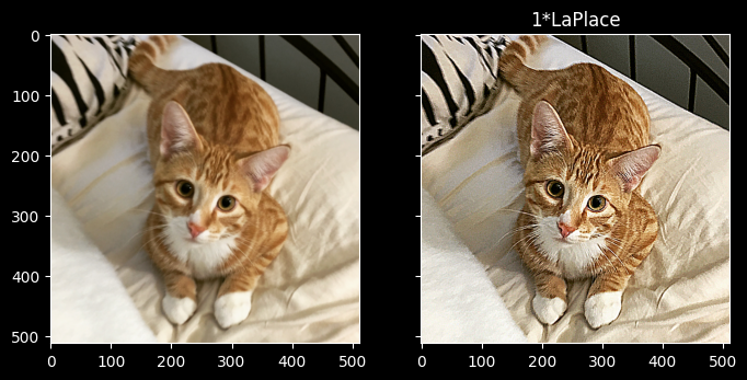

🧠 Further Efforts¶

So far, we’ve used a simple $3 \times 3$ Laplacian kernel. These problems explore the alternatives, and the scale at which we look for edges.

Four neighbors or eight? Repeat the sharpening with the 4-neighbor kernel described above (4 at the center, -1 at the four direct neighbors, 0 at the corners). How does the result differ from the 8-neighbor version? Look in particular at diagonal edges and at the overall strength of the effect.
Guidance: Use the same addLap approach and the same fractions, and compare with vis_pair so you can zoom into the same region of both.
The Laplacian at different scales. The Laplacian can be computed at different scales using Gaussian derivatives, the Laplacian of Gaussian, which lets us enhance detail at a coarser or finer level:
```
from scipy.ndimage import gaussian_laplace
I_log = np.stack([gaussian_laplace(I[...,i], sigma=2) for i in range(3)], axis=-1)
```
Add different amounts of this to the original image, as we did before, at sigma of 1, 2 and 4. How do the edges detected at sigma=1 differ from those at sigma=2 or sigma=4? What happens to fine details versus coarse structures as sigma grows?
Guidance: Watch the sign: gaussian_laplace computes the Laplacian itself, while our laplace_h is its negative (chosen so that we could add it). Also check the range of I_log with arr_info at each sigma: the response gets weaker as sigma grows, so a fair comparison needs a different fraction at each scale (multiplying by $\sigma^2$ is the standard fix). See filters_explore3D for what these kernels look like.
Two sliders. Write a version of addLap that takes both a sigma and a fraction, and build an interactive figure with a slider for each, to explore the scale and amount of sharpening together.
Guidance: Follow the slider pattern above, with one update function observed by both sliders. Recomputing gaussian_laplace on every slider move is slow, so precompute the response for a handful of sigma values and let that slider choose among them.