Exploring spatial filtering, low pass - imageprocessing-awesome

Preview: Exploring spatial filtering, low pass

Joshua Stough DIP 3.4 and 3.5 on spatial filtering and low-pass. See correlate

Here we’re going to look at a couple of spatial filters that reduce high frequency information. In other words, they blur the image.

First is a simple averaging, as we’ve done before.
Second is a Gaussian, which gives more weight to pixels closer to the center and less farther away. The Gaussian has better properties with respect to frequency information. We’ve seen Gaussian histograms, but you can read more about them in DIP 2.6.

%matplotlib inline
import matplotlib.pyplot as plt
import numpy as np

# For spatial filtering/operations
from scipy.ndimage import (correlate,
                           convolve)

# For importing from alternative directory sources
import sys  
sys.path.insert(0, '../dip_utils')

from matrix_utils import (arr_info,
                          make_linmap)
from vis_utils import (vis_rgb_cube,
                       vis_hists,
                       vis_pair)

from skimage.filters import *

plt.style.use('dark_background')

I = plt.imread('../dip_pics/cat_small.png').astype('float')
arr_info(I)

((512, 512, 4), dtype('float64'), np.float64(0.0), np.float64(1.0))

vis_hists(I)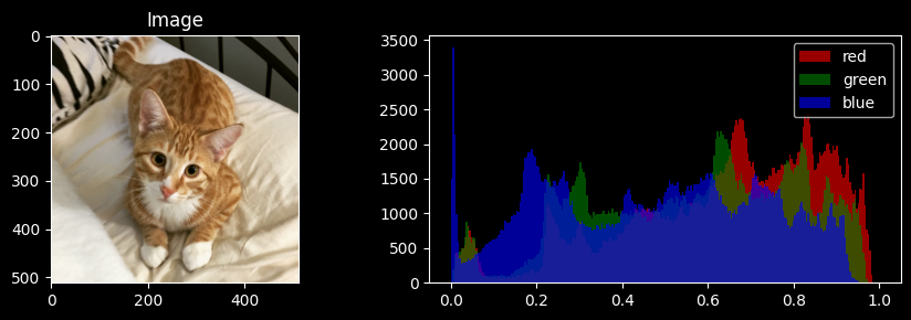

# The image includes an alpha channel that we're not going to need.
I = I[...,:3].copy()
arr_info(I)

((512, 512, 3),
 dtype('float64'),
 np.float64(0.0),
 np.float64(0.9882352948188782))

Low-pass filtering, or blurring, involves averaging neighborhoods of pixels,¶

thereby reducing the difference between neighboring pixels. We can do this in a number of ways. We’ve already seen local, equal weight averaging. We’re going to use a relatively large kernel size (filter size) to see the differences between the filters.

Note also, we’ll apply the filter to each channel separately. Zoom in on the figure to see the local differences.

mean_h = np.ones((11,11))/121
# mean_h

Correlation, kernels, and normalization¶

correlate slides the kernel (or filter, or mask) $h$ over the image $f$ . At each pixel it computes a weighted sum of the neighborhood under the kernel, with the kernel values as the weights. For a kernel of size $(2a+1) \times (2b+1)$ centered on the pixel:

g(r, c) = \sum_{s=-a}^{a} \sum_{t=-b}^{b} h(s, t)\, f(r+s, c+t)

Our mean_h is $11 \times 11$ with every entry $\frac{1}{121}$ , so $g$ is just the average of the $11 \times 11$ neighborhood. The weights sum to 1, which is what keeps the overall brightness unchanged: a region of constant intensity stays exactly the same. A kernel whose weights summed to 2 would also double the brightness.

A few practical details:

Convolution is the same operation with the kernel flipped ( $f(r-s, c-t)$ instead of $f(r+s, c+t)$ ). It’s the version with the nice mathematical properties, as we’ll see with the Fourier transform. For symmetric kernels like both of ours, correlation and convolution give identical results.
Borders: near the edge of the image, part of the kernel hangs off the image. scipy.ndimage.correlate handles this by default by reflecting the image at its border (mode='reflect'). Other choices are padding with zeros (mode='constant', which darkens the borders of a blurred image) or repeating the edge pixel (mode='nearest').
Cost: an $11 \times 11$ kernel means 121 multiply-adds per pixel per channel. Large blurs get expensive, which is one motivation for separable filters (below) and for filtering in the frequency domain.

I_localAverage11 = np.stack([correlate(I[...,i], mean_h) for i in range(3)], axis=-1)

vis_pair(I, I_localAverage11)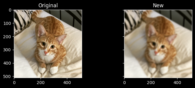

We can also try a weighted average that more highly weights¶

the pixels in the center of the neighborhood. A Gaussian is a good choice here.

from scipy.signal.windows import gaussian
gaus_h = gaussian(11, std=2, sym=True) # A Gaussian with std 1 symmetric about the size M.
# The result is a 1-d thing. take it's outer product to make a 2d thing.
gaus_h = np.outer(gaus_h, gaus_h)
gaus_h = gaus_h/gaus_h.sum()

The 2D Gaussian kernel is built as the outer product of a 1D Gaussian with itself: $h(s,t) = g(s)\,g(t)$ . A kernel like this is called separable. Filtering with it is equivalent to filtering every row with the 1D $g$ and then every column with $g$ again, which costs $11 + 11 = 22$ operations per pixel instead of 121. (The box filter is separable too.) We divide by the sum so that, as with the average, the weights add to 1.

# plot the two filter types
plt.figure()
plt.plot(gaus_h[5,:], label='Gaussian')
plt.plot(mean_h[5,:], label='Average')
plt.legend()
plt.suptitle('Different local filters');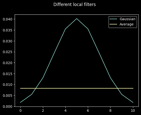

# Or consider in 2D.
vis_pair(gaus_h, mean_h, first_title='Gaussian', second_title='Average')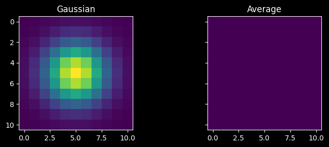

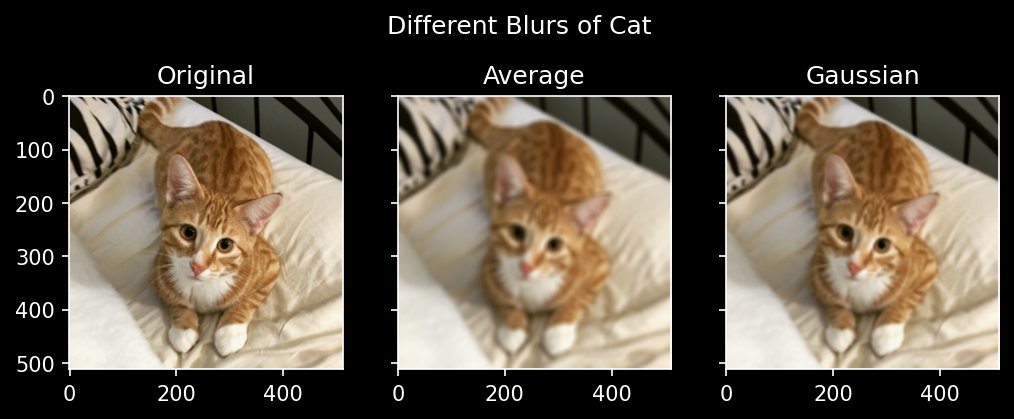
I_localGaussian11 = np.stack([correlate(I[...,i], gaus_h) for i in range(3)], axis=-1)

# Vis all three.
f, ax = plt.subplots(1,3, figsize=(8,3), sharex=True, sharey=True)
ax[0].imshow(I)
ax[0].set_title('Original')

ax[1].imshow(I_localAverage11)
ax[1].set_title('Average')

ax[2].imshow(I_localGaussian11)
ax[2].set_title('Gaussian')

plt.suptitle('Different Blurs of Cat');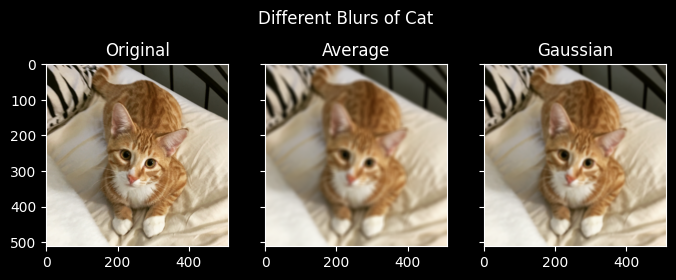

Beyond the amount of blur, there’s a difference in its character, though on a natural photo like this one it’s subtle. The box filter weights every pixel in its square equally and then cuts off abruptly. A Gaussian’s weights fall off smoothly and evenly in every direction, which is much closer to how an out-of-focus lens blurs. In frequency terms, the Gaussian is a much cleaner low-pass filter. It attenuates fine detail smoothly, while the box filter lets some fine, regular patterns leak back through, and on striped or checkered textures that can produce visible artifacts. We’ll make that precise in the Fourier chapter.

Let’s consider a midline through the image, and see what the¶

two filters did to the intensity values.

# Let's look at a midline through the image.
s = I.shape

f, ax = plt.subplots(1,2, figsize=(8,4))
ax[0].imshow(I)
ax[0].hlines(s[0]//2, xmin=0, xmax=s[1], color='r')
ax[0].set_title('Sample red channel from line.')

ax[1].plot(I[s[0]//2,:,0], label='Original')
ax[1].plot(I_localAverage11[s[0]//2,:,0], label='Average')
ax[1].plot(I_localGaussian11[s[0]//2,:,0], label='Gaussian')
ax[1].legend(loc='lower right');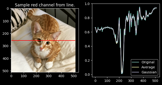

Along a single row, both filters follow the broad shape of the intensity profile while shaving off the narrow spikes (fur texture, the sharp edges of the eye). This is “low-pass” in action: slow variation passes through, rapid variation is attenuated. The box average flattens the spikes more, consistent with its wider effective width.

Interactive Visualization¶

We’re going to interactively visualize the Gaussian blur as you change the sigma/width of the gaussian.

See jupyter-matplotlib

from scipy.signal.windows import gaussian
def make_gaus(size=25, sig=1):
    gaus_h = gaussian(size, std=sig, sym=True) # A Gaussian with std 1 symmetric about the size M.
    # The result is a 1-d thing. take it's outer product to make a 2d thing.
    gaus_h = np.outer(gaus_h, gaus_h)
    gaus_h = gaus_h/gaus_h.sum()
    return gaus_h

from ipywidgets import VBox, FloatSlider, FloatLogSlider

sig = 0.5
gaus_h = make_gaus(sig=sig)
I_g = np.stack([correlate(I[...,i], gaus_h) for i in range(3)], axis=-1)


pass  # (static) plt.ioff()
plt.clf()

# https://ipywidgets.readthedocs.io/en/stable/examples/Widget%20List.html#FloatLogSlider
slider = FloatSlider(
    orientation='horizontal',
    value=0.5,
    min=0.5,
    max=20.0,
    step=0.5,
    description='Sig'
)

fig_args = {'num':' ', 'frameon':True}
fig, ax = plt.subplots(1,3, figsize=(10,3), **fig_args) 

# display artists I'll update
adisp = ax[0].imshow(I)
hdisp = ax[1].imshow(gaus_h, cmap='magma', vmin=0, vmax=gaus_h.max())
gdisp = ax[2].imshow(I_g)

htext = ax[1].set_title(f'Sig {sig:.3f}')
gtext = ax[2].set_title(f'Sig {sig:.3f}')


def update_image(change):
    global I, I_g, gaus_h, adisp, hdisp, gdisp, htext, gtext
    sig = change.new
    gaus_h = make_gaus(sig=sig)
    I_g = np.stack([correlate(I[...,i], gaus_h) for i in range(3)], axis=-1)
    
    
    hdisp.set_array(gaus_h)
    # need to reset the color limits each time since gaus_h is changing a lot. 
    hdisp.set_clim(0.0,gaus_h.max()) 
    htext.set_text(f'Sig {sig:.3f}')
    
    gdisp.set_array(I_g)
    gtext.set_text(f'Sig {sig:.3f}')
    
    fig.canvas.draw()
    fig.canvas.flush_events()

slider.observe(update_image, names='value')

pass  # (static) VBox([slider, fig.canvas])

<Figure size 640x480 with 0 Axes>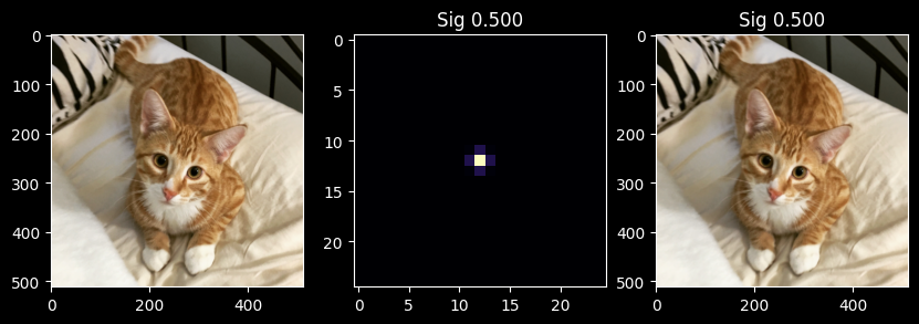

As you increase $\sigma$ , the kernel spreads out and the blur grows. But notice that make_gaus always builds a $25 \times 25$ kernel. A Gaussian has most of its weight within about $3\sigma$ of the center, so a kernel needs to be about $6\sigma + 1$ wide to hold it. Past roughly $\sigma = 4$ , our kernel cuts off the Gaussian’s tails. By $\sigma = 20$ the kernel is nearly flat across its 25 pixels, so we’re really applying something close to a $25 \times 25$ box filter, and the image stops getting blurrier. Watch the kernel display in the middle panel as you slide.