Gradient Maps and Edge Detection - imageprocessing-awesome

DRAFT, not finalized. This chapter is new and still under review.

stough 202-

Preview: Gradient Maps and Edge Detection

Gradient magnitude and direction
Noise, and why we smooth first
Canny edge detection, step by step
Interactive Canny
🔨 Your Turn: Tune Canny on a Noisy Image
🧠 Further Efforts

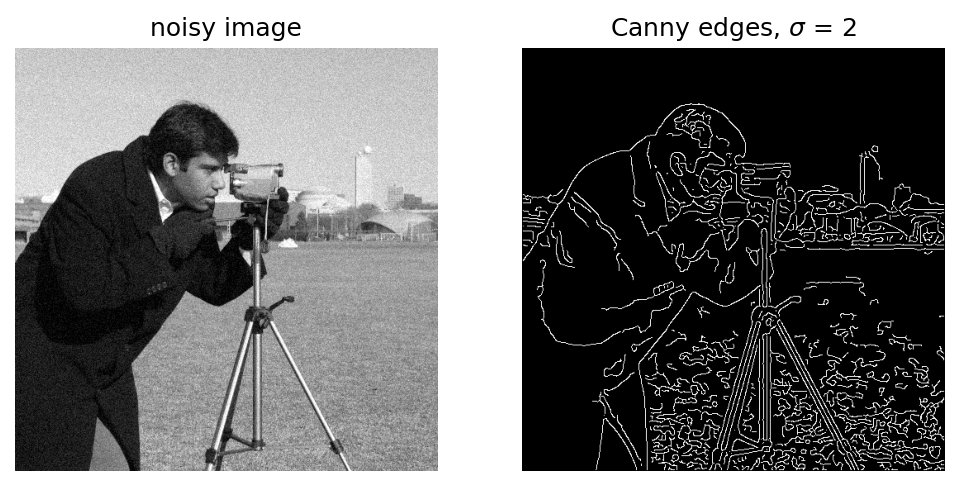
In Spatial Operations we computed the gradient magnitude of an image with the Sobel kernels: a map of how steeply the intensity changes at every pixel, bright at edges and dark in flat regions. That’s a picture of edges, but it isn’t yet an answer to “where are the edges?” Its edges are several pixels thick, it responds weakly to faint edges and strongly to noise, and it says nothing about which pixels belong to the same edge.

An edge detector turns the gradient into a yes/no decision per pixel: a thin, connected outline. In this notebook we’ll build the most famous one, Canny’s (1986), from pieces we mostly already have, and then compare it with scikit-image’s implementation.

%matplotlib inline
import matplotlib.pyplot as plt
import numpy as np
from scipy.ndimage import gaussian_filter, sobel, label
from skimage import data
from skimage.color import hsv2rgb
from skimage.feature import canny
from skimage.util import img_as_float
from ipywidgets import VBox, FloatSlider

# For importing from alternative directory sources
import sys
sys.path.insert(0, '../dip_utils')

from matrix_utils import arr_info
from vis_utils import vis_pair, vis_triple

Gradient Magnitude and Direction¶

We’ll use the classic camera test image that ships with scikit-image, as floats in $[0,1]$ . The Sobel kernels estimate the derivatives in $x$ (along the columns) and $y$ (down the rows). scipy.ndimage.sobel applies them for us: axis=1 differentiates along the columns, axis=0 along the rows.

The two derivatives together form the gradient vector $\nabla I = \langle G_x, G_y \rangle$ at every pixel. It has a length and a direction:

|\nabla I| = \sqrt{G_x^2 + G_y^2}, \qquad \theta = \operatorname{atan2}(G_y, G_x).

The gradient points in the direction of steepest increase in intensity, so it is perpendicular to the edge: across it, from dark to bright.

I = img_as_float(data.camera())
arr_info(I)

Gx = sobel(I, axis=1)    # derivative along x (columns)
Gy = sobel(I, axis=0)    # derivative along y (rows, pointing down)
mag = np.hypot(Gx, Gy)   # same as np.sqrt(Gx**2 + Gy**2)
theta = np.arctan2(Gy, Gx)
arr_info(mag)

((512, 512), dtype('float64'), np.float64(0.0), np.float64(3.6474762569457115))

To see the direction, we can borrow from the Color chapter: hue is an angle too. Below, each pixel’s hue is its gradient direction and its value (brightness) is its gradient magnitude, so flat regions are black and edges are colored by which way they face.

hue = (theta + np.pi) / (2 * np.pi)                 # direction, mapped to [0, 1]
value = np.clip(mag / np.percentile(mag, 99), 0, 1)  # magnitude, with the brightest 1% saturated
direction_rgb = hsv2rgb(np.stack([hue, np.ones_like(hue), value], axis=-1))

vis_triple(I, mag, direction_rgb, cmap='gray', figsize=(10, 3.5),
           first_title='camera', second_title='gradient magnitude',
           third_title='direction as hue', show_ticks=False)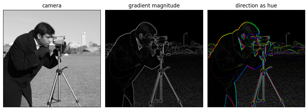

In the magnitude image (middle), the outline of the photographer, the camera and tripod, and the buildings in the background are bright; the sky and the smooth parts of his coat are dark. Notice, though, that the grass is covered in a fine speckle: lots of small changes, each a little bit of “edge”.

In the direction image (right), the two sides of a thin object, like a tripod leg, have opposite colors. The gradient points toward the brighter side, so on either side of a thin bright leg it points in opposite directions, toward the leg. Long straight edges keep a single color along their length, because their direction doesn’t change.

Noise, and Why We Smooth First¶

Derivatives amplify noise. A derivative measures the difference between neighbors, and noise is exactly where neighbors differ for no good reason. Let’s add a little Gaussian noise to the image, of a standard deviation of only 5% of the intensity range, and look at the gradient magnitude again.

rng = np.random.default_rng(0)
I_noisy = np.clip(I + rng.normal(0, 0.05, I.shape), 0, 1)

mag_noisy = np.hypot(sobel(I_noisy, axis=1), sobel(I_noisy, axis=0))
vis_pair(I_noisy, mag_noisy, cmap='gray', figsize=(8, 4), show_ticks=False,
         first_title='5% noise', second_title='gradient magnitude')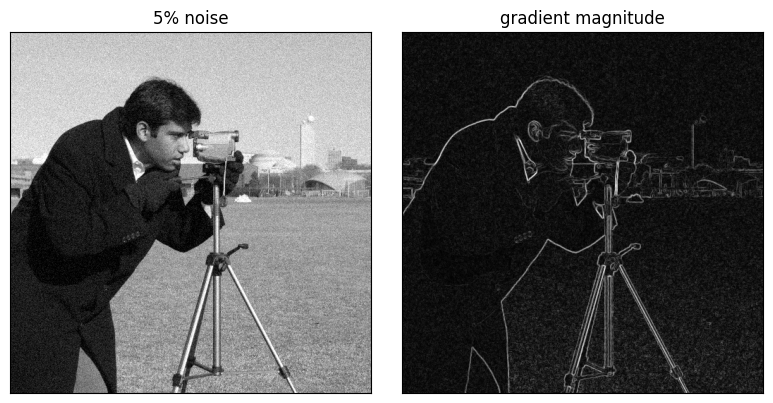

The noise is barely noticeable in the image, but it’s all over the gradient magnitude. In the sky (the top-left corner), the average magnitude jumps tenfold, from about 0.02 to 0.23, and its brightest noise pixels are as strong as many of the real edges. Any threshold low enough to keep the faint edges would also keep thousands of noise pixels.

The cure is to smooth before differentiating, with a Gaussian low-pass filter. The noise averages out, while edges, which extend over many pixels, survive. And because convolution is associative, smoothing and then differentiating is the same as convolving once with the derivative of a Gaussian:

\frac{\partial}{\partial x}\left(g_\sigma * I\right) = \left(\frac{\partial g_\sigma}{\partial x}\right) * I.

That is the kernel we looked at as a 3D height map in filters_explore3D. The Gaussian’s $\sigma$ sets the scale of the edges we’re looking for: larger $\sigma$ ignores more noise and fine texture, and keeps only the broad outlines.

fig, ax = plt.subplots(1, 3, figsize=(10, 3.5), sharex=True, sharey=True)
for a, sigma in zip(ax, [1, 2, 4]):
    smoothed = gaussian_filter(I_noisy, sigma)
    a.imshow(np.hypot(sobel(smoothed, axis=1), sobel(smoothed, axis=0)), cmap='gray')
    a.set_title(rf'smoothed with $\sigma = {sigma}$')
    a.set_axis_off()
plt.tight_layout()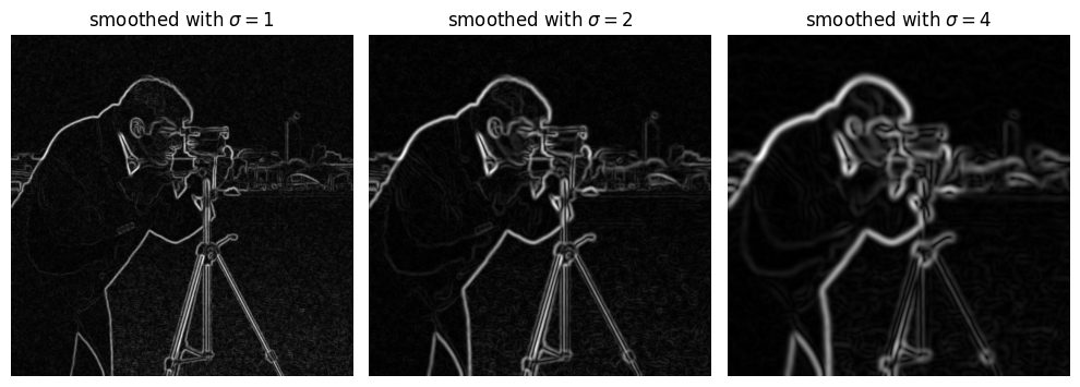

At $\sigma = 1$ the sky is already much quieter, and by $\sigma = 2$ its average magnitude is nearly back to that of the clean image. By $\sigma = 4$ the noise is gone and the grass texture has faded to faint blobs, but the edges have become wide and soft, and the tripod’s two thin legs are blurring together. There’s no single right $\sigma$ : it depends on how noisy the image is and how fine the edges you care about are. This trade-off between noise suppression and localization is fundamental, and Canny’s method has a $\sigma$ parameter for exactly this reason.

Canny Edge Detection, Step by Step¶

Canny’s detector has four steps:

Smooth and differentiate: Gaussian smoothing, then Sobel, giving the gradient magnitude and direction. (Done.)
Non-maximum suppression: thin each edge to a one-pixel-wide ridge.
Double threshold: classify the survivors as strong or weak edges, and discard the rest.
Hysteresis: keep the weak edges only where they connect to strong ones.

We’ll work with the noisy image at $\sigma = 2$ .

sigma = 2
smoothed = gaussian_filter(I_noisy, sigma)
Gx = sobel(smoothed, axis=1)
Gy = sobel(smoothed, axis=0)
mag = np.hypot(Gx, Gy)
theta = np.arctan2(Gy, Gx)
arr_info(mag)

((512, 512),
 dtype('float64'),
 np.float64(5.8702306506753004e-05),
 np.float64(1.2763935310629921))

Non-maximum suppression¶

Across an edge, the gradient magnitude rises and falls like a hill. The edge itself is the top of the hill, the one pixel where the magnitude is largest. Non-maximum suppression keeps a pixel only if its magnitude is at least as large as that of its two neighbors along the gradient direction, that is, across the edge. Pixels on the slopes of the hill are set to zero, leaving a thin ridge.

With only 8 neighbors to choose from, we round each gradient direction to the nearest of four: horizontal ( $0°$ ), the two diagonals ( $45°$ and $135°$ ), and vertical ( $90°$ ). A direction and its opposite share the same pair of neighbors, so angles only matter modulo $180°$ . Remember that $y$ points down, so a $45°$ gradient points down and to the right.

def non_max_suppression(mag, theta):
    '''Keep only pixels whose magnitude is a maximum along the gradient direction.'''
    angle = np.rad2deg(theta) % 180                  # direction modulo 180 degrees
    bins = (np.round(angle / 45) % 4).astype(int)    # 0: 0deg, 1: 45deg, 2: 90deg, 3: 135deg
    offsets = [(0, 1), (1, 1), (1, 0), (1, -1)]      # (row, col) step along each direction

    H, W = mag.shape
    padded = np.pad(mag, 1)
    out = np.zeros_like(mag)
    for b, (dr, dc) in enumerate(offsets):
        ahead = padded[1 + dr:1 + dr + H, 1 + dc:1 + dc + W]    # neighbor one step along the gradient
        behind = padded[1 - dr:1 - dr + H, 1 - dc:1 - dc + W]   # neighbor one step against it
        keep = (bins == b) & (mag >= ahead) & (mag >= behind)
        out[keep] = mag[keep]
    return out

thin = non_max_suppression(mag, theta)
vis_pair(mag, thin, cmap='gray', figsize=(8, 4), show_ticks=False,
         first_title=r'gradient magnitude, $\sigma = 2$', second_title='after non-maximum suppression')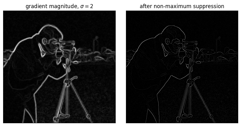

Rather than loop over pixels, non_max_suppression handles one direction at a time. Slicing the zero-padded magnitude array with an offset gives, for every pixel at once, the neighbor one step ahead (or behind) in that direction. keep then marks the pixels whose direction falls in this bin and that are at least as large as both neighbors.

Zoom in on the right-hand image: the wide, soft edges are now thin lines, one pixel wide. But every little noise bump in the sky is also the top of its own (tiny) hill, so the sky is full of short, faint ridges. That’s what thresholding is for.

Double threshold and hysteresis¶

A single threshold forces a bad choice: set it high and the faint parts of real edges break up; set it low and the noise ridges get in. Canny uses two thresholds instead:

pixels above the high threshold are strong edges, kept for sure;
pixels between the low and high thresholds are weak edges, kept only if they are connected to a strong edge, possibly through other weak pixels.

This last step is called hysteresis. A real edge usually has a strong part somewhere along it, and the weak parts of the same edge are connected to it. Noise ridges are short, isolated, and usually all weak. To find connections, we label the connected groups of weak-or-strong pixels with scipy.ndimage.label, counting diagonal neighbors as connected, and keep every group that contains at least one strong pixel.

low, high = 0.04, 0.10

def hysteresis(thin, low, high):
    strong = thin >= high
    candidates = thin >= low                                  # weak or strong
    groups, n = label(candidates, structure=np.ones((3, 3)))  # connected groups, 8-connectivity
    keep = np.unique(groups[strong])                          # the groups containing a strong pixel
    return np.isin(groups, keep[keep > 0])

strong = thin >= high
weak = (thin >= low) & ~strong
edges = hysteresis(thin, low, high)

# Show strong pixels in white and weak ones in red, next to the final result.
classes = np.zeros(I.shape + (3,))
classes[strong] = [1, 1, 1]
classes[weak] = [1, 0, 0]
vis_pair(classes, edges, cmap='gray', figsize=(8, 4), show_ticks=False,
         first_title='strong (white) and weak (red)', second_title='Canny edges')
print(f'{strong.sum()} strong pixels, {weak.sum()} weak, {edges.sum()} in the final edges')

11744 strong pixels, 22174 weak, 20078 in the final edges

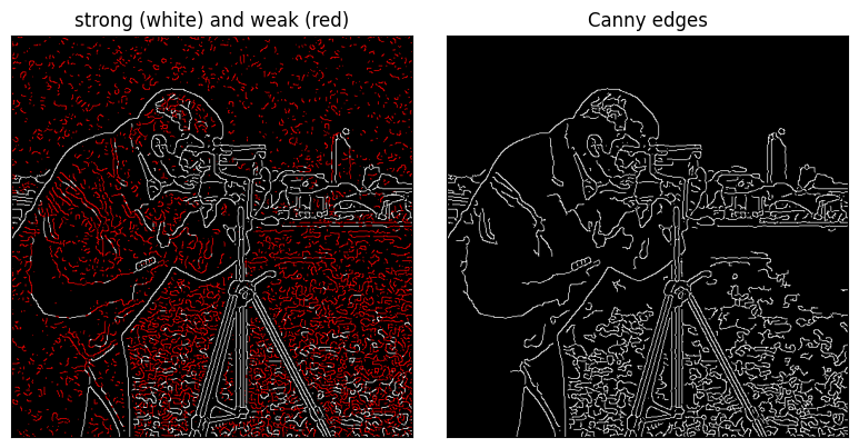
On the left, the strong pixels trace the main outlines, with gaps wherever the edge is faint, while weak pixels fill those gaps and also scatter across the sky and grass. On the right, hysteresis has kept the weak pixels that continue a strong edge and dropped the isolated ones: the outlines of the photographer, his camera and tripod are long and mostly unbroken, and the sky is empty.

The grass is another story. Its texture produces genuinely strong gradients at this scale, so Canny keeps much of it. These are real edges, just not ones we care about. A larger $\sigma$ or higher thresholds would remove them, at the cost of some detail elsewhere; you’ll get to try that below.

The thresholds here are in the units of the gradient magnitude (the Sobel kernels’ weights make it about 8 times the actual derivative). I chose them by looking at the result. Choosing thresholds automatically is a hard problem in general; one common rule of thumb sets them as percentiles of the gradient magnitude.

Comparing with scikit-image¶

skimage.feature.canny implements the same four steps. It smooths and differentiates the same way, so we can give it the same $\sigma$ and thresholds.

edges_sk = canny(I_noisy, sigma=sigma, low_threshold=low, high_threshold=high)

# Where do the two disagree?
diff = np.zeros(I.shape + (3,))
diff[edges & edges_sk] = [1, 1, 1]      # both
diff[edges & ~edges_sk] = [1, 0, 0]     # ours only
diff[~edges & edges_sk] = [0, 1, 1]     # scikit-image only
vis_pair(edges_sk, diff, cmap='gray', figsize=(8, 4), show_ticks=False,
         first_title='skimage.feature.canny', second_title='both (white), ours (red), skimage (cyan)')

print(f'ours: {edges.sum()} pixels, skimage: {edges_sk.sum()}, in both: {(edges & edges_sk).sum()}')

ours: 20078 pixels, skimage: 19084, in both: 17293

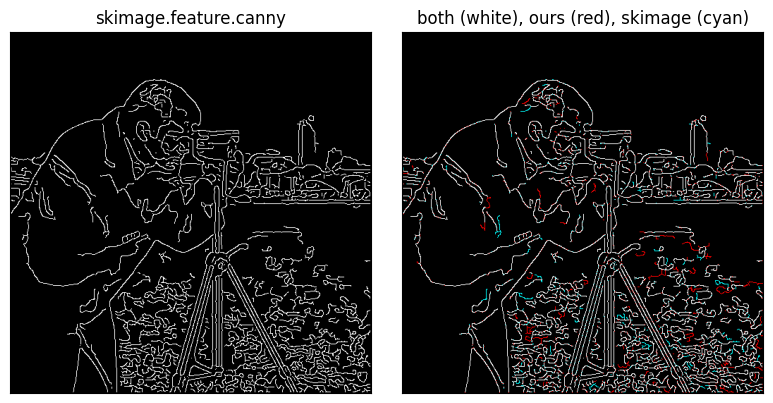
The two results trace the same outlines, and most of their edge pixels coincide. Along the main outlines they agree almost everywhere. Most of the disagreements are in the grass, where short fragments are kept by one and not the other, plus a few places where a line is shifted by a pixel. Two implementation details account for that. scikit-image doesn’t round the gradient direction to one of four bins: it interpolates the magnitude between the two nearest neighbors on each side, which places diagonal edges more precisely. It also handles the image border differently. Small differences in non-maximum suppression then change which weak pixels connect to strong ones.

Our couple of dozen lines of code reproduce the essentials of a classic algorithm. In practice, use the library version: it’s faster, better tested, and can choose thresholds from quantiles for you (use_quantiles=True).

Interactive Canny¶

Here’s canny with sliders for $\sigma$ and the high threshold (the low threshold is kept at half the high one). Try it on the clean and noisy images, by changing J below.

J = I_noisy   # or I

pass  # (static) plt.ioff()
sigma_slider = FloatSlider(value=2, min=0.5, max=6, step=0.25, description='sigma')
high_slider = FloatSlider(value=0.10, min=0.02, max=0.4, step=0.01, description='high')

fig, ax = plt.subplots(1, 2, figsize=(8, 4), sharex=True, sharey=True)
fig.canvas.header_visible = False
ax[0].imshow(J, cmap='gray')
edisp = ax[1].imshow(canny(J, sigma=2, low_threshold=0.05, high_threshold=0.10), cmap='gray')
for a in ax:
    a.set_axis_off()

def update(change):
    high = high_slider.value
    edisp.set_data(canny(J, sigma=sigma_slider.value, low_threshold=high / 2, high_threshold=high))
    fig.canvas.draw()
    fig.canvas.flush_events()

sigma_slider.observe(update, names='value')
high_slider.observe(update, names='value')

pass  # (static) VBox([sigma_slider, high_slider, fig.canvas])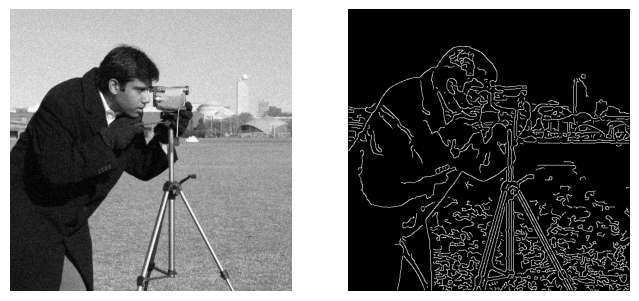

🔨 Your Turn: Tune Canny on a Noisy Image¶

Task: Choose an image with clear objects and add noise to it: Gaussian noise with a standard deviation of 0.1 (twice what we used), or a photo of your own taken in dim light. Find the Canny settings ( $\sigma$ , low and high thresholds) that best recover the outlines of the main objects while ignoring the noise. Show your best result, and one result each where $\sigma$ is clearly too small and clearly too large. In a few sentences, describe the trade-off you ran into.

Guidance:

Use the interactive figure above (set J to your noisy image) to explore, then record your settings and show the final results in ordinary figures.
Decide what a “good” result is before tuning: which outlines matter? Running canny on the clean image gives you a reference to compare against.
Change one parameter at a time. Which one mostly controls the noise speckle, and which mostly controls the gaps in real edges?
Check whether the ratio between the low and high thresholds matters, or only their overall level.

🧠 Further Efforts¶

Which way do edges face? Make a histogram of the gradient directions $\theta$ , weighted by magnitude so that strong edges count more, for a photo of a city street and for a photo of a forest or field. How do the two histograms differ, and why?
Guidance: np.histogram takes a weights argument. Directions that differ by $180°$ describe the same edge orientation, so you may want to fold $\theta$ into $[0°, 180°)$ .
Interpolated non-maximum suppression. Our non_max_suppression rounds the direction to one of four bins. Instead, estimate the magnitude at the exact point one pixel along the gradient by interpolating between the two nearest neighbors, as scikit-image does. Does it bring our result closer to canny’s?
Guidance: scipy.ndimage.map_coordinates with order=1 does bilinear interpolation at arbitrary positions, as in coord_ops. Compare the two by counting agreeing pixels, as above.
Edges in color. Two regions can have the same brightness but different hues, and then a grayscale edge detector misses the boundary between them. Design an edge detector for color images, and find (or make) an image where it finds an edge that grayscale Canny misses.
Guidance: One approach computes the gradient magnitude of each channel and combines them at every pixel. Which colorspace you work in matters; see the Color chapter.