Coordinate Operations Demo - imageprocessing-awesome

stough 202-

Every pixel’s coordinates
The rotation matrix
Inverse mapping
Why not forward mapping?
Rotating about the center, and interpolation

So far, our operations have changed pixel values: transfer functions map each intensity to a new intensity, and the pixel stays where it is. Coordinate operations (or geometric transforms) do the opposite: they move pixels around, as in rotation, scaling, shearing, or warping, while leaving their values alone. The trick is all in the bookkeeping, deciding for each pixel of the output image which pixel of the input should land there. This is the math behind every “rotate” button, and behind image registration, panoramas, and lens-distortion correction.

Without a linear algebra background, a lot of this is going to take time to cook. Please peruse the following awesome sources:

The incredible Khan Academy, with three integrated units up through orthogonal projections.
BYJU’s introduction
The better explained series post on the topic.

%matplotlib inline
import matplotlib.pyplot as plt
import numpy as np

# For spatial filtering/operations
from scipy.ndimage import (correlate,
                           convolve)

# For importing from alternative directory sources
import sys  
sys.path.insert(0, '../dip_utils')

from matrix_utils import (arr_info,
                          make_linmap)
from vis_utils import (vis_rgb_cube,
                       vis_hists,
                       vis_pair)

I = plt.imread('../dip_pics/happy128.png')
vis_hists(I)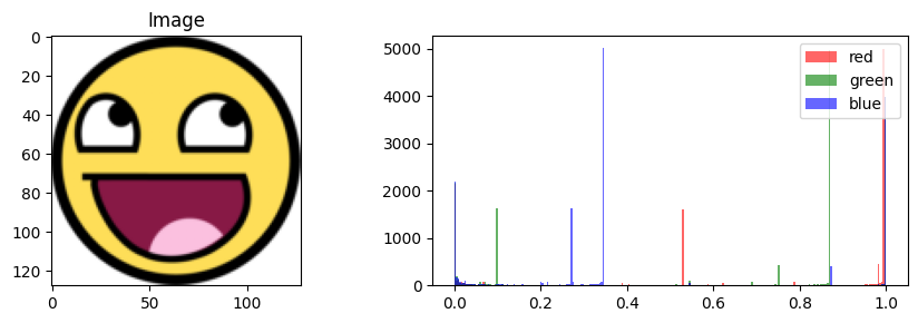

Every Pixel’s Coordinates¶

Our test image is a small $128 \times 128$ RGB smiley face. To move pixels around with matrix math, we first need the coordinates of every pixel as a list of 2D points. np.meshgrid builds two arrays the size of the image, one holding each pixel’s row index and one its column index. (With these arguments, x ends up holding the row index and y the column, matching how we index an image as I[row, col]. Look at the two printed arrays below to confirm.)

arr_info(I)

((128, 128, 3), dtype('float32'), np.float32(0.0), np.float32(1.0))

y, x = np.meshgrid(range(I.shape[0]), range(I.shape[1]))

array([[  0,   0,   0, ...,   0,   0,   0],
       [  1,   1,   1, ...,   1,   1,   1],
       [  2,   2,   2, ...,   2,   2,   2],
       ...,
       [125, 125, 125, ..., 125, 125, 125],
       [126, 126, 126, ..., 126, 126, 126],
       [127, 127, 127, ..., 127, 127, 127]])

array([[  0,   1,   2, ..., 125, 126, 127],
       [  0,   1,   2, ..., 125, 126, 127],
       [  0,   1,   2, ..., 125, 126, 127],
       ...,
       [  0,   1,   2, ..., 125, 126, 127],
       [  0,   1,   2, ..., 125, 126, 127],
       [  0,   1,   2, ..., 125, 126, 127]])

coords = np.stack([x.ravel(), y.ravel()], axis=0)
arr_info(coords)

((2, 16384), dtype('int64'), np.int64(0), np.int64(127))

coords is a $2 \times 16384$ matrix: each column is one pixel’s $(row, col)$ position. Stacking all the points as columns of one matrix lets us transform every pixel with a single matrix multiplication.

The Rotation Matrix¶

Rotating a 2D point by an angle $\theta$ about the origin is a linear transformation, so it can be written as a $2 \times 2$ matrix:

\mathbf{T} = \begin{bmatrix} \cos\theta & -\sin\theta \\ \sin\theta & \cos\theta \end{bmatrix}, \qquad \begin{bmatrix} r' \\ c' \end{bmatrix} = \mathbf{T} \begin{bmatrix} r \\ c \end{bmatrix}

One way to see where this comes from: the columns of a matrix are where it sends the basis vectors. The first column, $\langle \cos\theta, \sin\theta \rangle$ , is where $\langle 1, 0 \rangle$ lands after rotating by $\theta$ , and the second, $\langle -\sin\theta, \cos\theta \rangle$ , is where $\langle 0, 1 \rangle$ lands. Every other point is a combination of those two, so it rotates along with them.

Rotation = lambda theta: np.array([[np.cos(theta), -np.sin(theta)], [np.sin(theta), np.cos(theta)]])

T = Rotation(np.pi/4)

array([[ 0.70710678, -0.70710678],
       [ 0.70710678,  0.70710678]])

Tinv = T.transpose()

Rotation matrices are orthogonal: their columns are perpendicular unit vectors. That makes the inverse especially cheap, since $\mathbf{T}^{-1} = \mathbf{T}^\intercal$ . Undoing a rotation by $\theta$ is the same as rotating by $-\theta$ , and if you substitute $-\theta$ into $\mathbf{T}$ you get exactly its transpose.

Tinv

array([[ 0.70710678,  0.70710678],
       [-0.70710678,  0.70710678]])

Inverse Mapping: Old Coordinates from New¶

Here’s the key idea. We want an output image J that is I rotated by $\mathbf{T}$ . The natural way to think of it is “take each pixel of I and send it to its new location”. But we’ll do it the other way around: for each pixel location in the output J, ask where it came from in I:

\begin{bmatrix} r \\ c \end{bmatrix}_{old} = \mathbf{T}^{-1} \begin{bmatrix} r' \\ c' \end{bmatrix}_{new}, \qquad J(r', c') = I(r_{old}, c_{old})

So coords now plays the role of the new (output) coordinates, and multiplying by Tinv gives the old (input) coordinate each output pixel should copy from.

oldcoords = np.matmul(Tinv, coords)

Two complications. First, many of the old coordinates fall outside the input image, at negative rows or columns, or past 127. Those output pixels have no source and stay black. Second, the old coordinates are generally not integers: the source of an output pixel might be “row 37.4, column 81.9”. We need some rule to pick a value there; this is called interpolation.

arr_info(oldcoords)

((2, 16384),
 dtype('float64'),
 np.float64(-89.80256121069152),
 np.float64(179.60512242138307))

J = np.zeros_like(I)
arr_info(J)

((128, 128, 3), dtype('float32'), np.float32(0.0), np.float32(0.0))

valid = np.logical_and(np.min(oldcoords, axis=0)>=0, np.max(oldcoords, axis=0)<128)

valid is a boolean mask over all 16384 output pixels: True where both old coordinates land inside the input image. Only about 42% do, because we’re rotating about the top-left corner (the origin $(0,0)$ ), so most of the rotated image swings up and out of the frame.

arr_info(valid)

((16384,), dtype('bool'), np.False_, np.True_)

rounded_old = np.floor(oldcoords).astype('int')
J[coords[0,valid], coords[1,valid],:] = I[rounded_old[0,valid],rounded_old[1,valid],:]

For interpolation, this cell just truncates each old coordinate down to an integer (np.floor), copying the value of a nearby input pixel. (Rounding with np.round would pick the truly nearest pixel, which is called nearest-neighbor interpolation.) Then one line of fancy indexing copies all the valid pixels at once: output locations coords[:, valid] receive the input values at rounded_old[:, valid].

plt.figure()
plt.imshow(J, interpolation='none', aspect=1.0)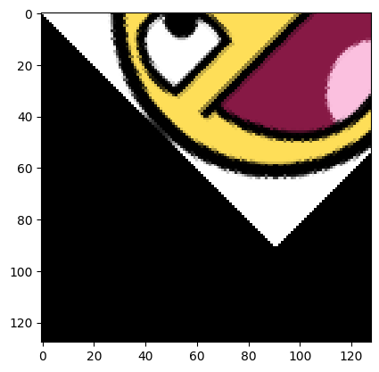

There’s our smiley, rotated $45°$ about the top-left corner, with only the part that stayed in frame visible. Because rows increase downward on screen, the rotation appears counterclockwise on screen.

arr_info(valid)

((16384,), dtype('bool'), np.False_, np.True_)

Why Not Forward Mapping?¶

Why go through the trouble of the inverse? Let’s try the “natural” way and see what goes wrong. This time we’ll rotate by $30°$ and also scale up by 1.5, sending each input pixel to its rounded output location.

center = np.array([[63.5], [63.5]])          # the middle of a 128x128 image
A = 1.5 * Rotation(np.pi/6)                  # rotate 30 degrees and scale by 1.5

# Forward: each input pixel goes to its (rounded) new location.
newcoords = np.round(np.matmul(A, coords - center) + center).astype('int')
ok = np.logical_and(np.min(newcoords, axis=0) >= 0, np.max(newcoords, axis=0) < 128)

J_forward = np.zeros_like(I)
J_forward[newcoords[0, ok], newcoords[1, ok], :] = I[coords[0, ok], coords[1, ok], :]

plt.figure(figsize=(3,3))
plt.imshow(J_forward, interpolation='none')
plt.title('Forward mapping');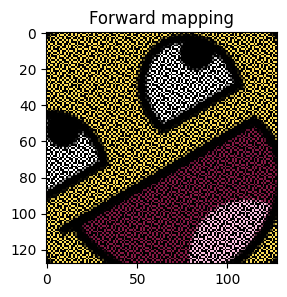

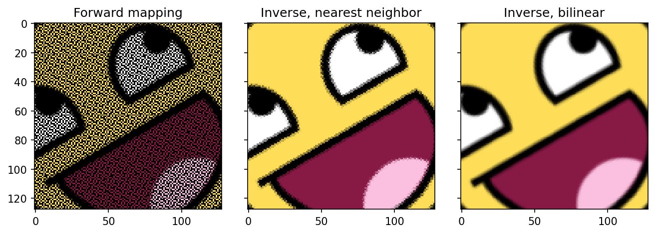
The result is riddled with holes. Scaling up by 1.5 means the output has more pixels in the region than the input has pixels to send there, so many output pixels are never hit by anyone. (In other places, two input pixels can round to the same output pixel, and one simply overwrites the other.) Forward mapping gives no guarantee that every output pixel receives exactly one value.

Inverse mapping makes that guarantee automatically: we loop over output pixels, so each one gets exactly one value. That’s why essentially every image-warping library, including skimage.transform.warp, works with the inverse map.

Rotating About the Center, and Interpolation¶

Notice that cell also rotated about the image’s center instead of the corner. To do that: shift the coordinates so the center is at the origin, apply the matrix, and shift back:

\mathbf{p}' = \mathbf{A}(\mathbf{p} - \mathbf{c}) + \mathbf{c} \qquad \Longrightarrow \qquad \mathbf{p} = \mathbf{A}^{-1}(\mathbf{p}' - \mathbf{c}) + \mathbf{c}

Now let’s do the same rotate-and-scale properly with inverse mapping. We’ll also compare two kinds of interpolation. Nearest neighbor rounds the old coordinate and copies that one pixel. Bilinear takes a distance-weighted average of the four input pixels surrounding the old coordinate. scipy.ndimage.map_coordinates does exactly this lookup for us: hand it an image and a list of (possibly fractional) old coordinates, and order=0 gives nearest neighbor, order=1 bilinear.

from scipy.ndimage import map_coordinates

# Inverse: for each output pixel, where did it come from?
oldcoords2 = np.matmul(np.linalg.inv(A), coords - center) + center

def warp_channels(I, oldcoords, order):
    return np.stack([map_coordinates(I[..., k], oldcoords, order=order, cval=0).reshape(I.shape[:2])
                     for k in range(I.shape[2])], axis=-1)

J_nearest = warp_channels(I, oldcoords2, order=0)
J_bilinear = warp_channels(I, oldcoords2, order=1)

f, ax = plt.subplots(1, 3, figsize=(9,3), sharex=True, sharey=True)
for a, Jx, title in zip(ax, [J_forward, J_nearest, J_bilinear],
                        ['Forward mapping', 'Inverse, nearest neighbor', 'Inverse, bilinear']):
    a.imshow(np.clip(Jx, 0, 1), interpolation='none')
    a.set_title(title)
plt.tight_layout()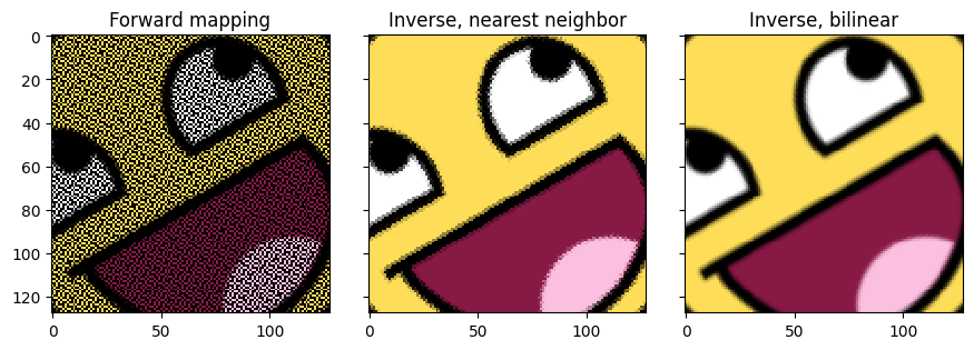

Inverse mapping fills every pixel. Zoom in on the edges of the eyes and mouth to compare the two interpolations: nearest neighbor leaves jagged, stair-stepped edges, since each output pixel copies one input pixel whole. Bilinear interpolation blends neighbors, giving smoother edges at the cost of a little blur. Higher-order interpolation (bicubic, order=3) blends a larger neighborhood for a sharper, smoother result, at more computational cost. The same trade-off showed up when we resampled images to change their resolution. That was a coordinate operation too, just a scaling.

Every geometric transform works this way: compute the inverse map from output to input coordinates, then interpolate. Only the map changes. Rotation, scaling and shearing are all $2 \times 2$ matrices; adding a translation gives the affine transforms; and more general warps can use any function at all.