stough, 202-
Trying out alternative color picking schemes for a 256-color palette... The way I chose in color_clustering is k-means, which works pretty well. Some other ideas:
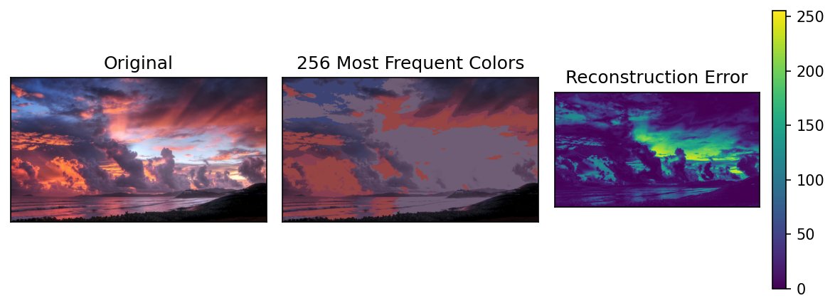
Pick the 256 most frequent colors (this is the one I’m doing here)
replace very rare colors with nearby more common ones until you get to 256? Interesting, maybe hard to implement...?
compare every pixel with neighbor. take median (really just average), then pick the 256 most common medians...That seems overly complicated
%matplotlib inline
import scipy.cluster.vq as vq
import matplotlib.pyplot as plt
import numpy as np

# For importing from alternative directory sources
import sys
sys.path.insert(0, '../dip_utils')

from matrix_utils import arr_info
from vis_utils import (vis_rgb_cube,
                       vis_hists,
                       vis_pair)
"""
Computes a colormap (256x3) of the most frequent colors.
I'm assuming the image is in the uint8 [0,255] range.
Displays the vector quantized image.
"""
I = plt.imread('../dip_pics/skyandsea.jpg')
allcolors = I[...,0].astype('uint32').ravel() \
+ 256*I[...,1].astype('uint32').ravel() \
+ 256**2*I[...,2].astype('uint32').ravel()
#allcolors is the 1d value for each pixel. Every R,G,B goes to a unique number
#in [0, 256**3-1]
uniques = np.unique(allcolors)
hist, bins = np.histogram(allcolors, bins = np.append(uniques, [256**3]))
sortedinds = np.argsort(hist)
#sortedinds goes from least to most popular color values.
#https://docs.scipy.org/doc/scipy/reference/generated/scipy.cluster.vq.vq.html
temp = bins[sortedinds[-256:]]
code_book = np.zeros((256, 3))
code_book[:,0] = temp%256
temp = temp//256
code_book[:,1] = temp%256
temp = temp//256
code_book[:,2] = temp
#code_book is 256x3, now we need to assign every pixel to one of those
#256.
X = np.concatenate([np.expand_dims(IC, axis = 1) for IC in
[I[...,0].ravel(), I[...,1].ravel(), I[...,2].ravel()]], axis = 1)
#X is N*Mx3
#Call vq to quantize the pixels X by the code_book.
color_codes, dist = vq.vq(X, code_book)
#Now reconstruct the image with the 256 most popular colors.
Ir = np.zeros(I.shape)
Ir[...,0] = np.reshape(code_book[color_codes, 0], I.shape[:2])
Ir[...,1] = np.reshape(code_book[color_codes, 1], I.shape[:2])
Ir[...,2] = np.reshape(code_book[color_codes, 2], I.shape[:2])
Ir = Ir.astype('uint8')
#Visualize
f, ax = plt.subplots(1,3, figsize=(8,3))
ax[0].imshow(I)
ax[0].set_title('Original')
ax[1].imshow(Ir)
ax[1].set_title('256 Most Frequent Colors')
#On how to put the colorbar on a subplot:
#https://matplotlib.org/examples/images_contours_and_fields/pcolormesh_levels.html
pic = ax[2].imshow(np.reshape(dist, I.shape[:2]))
f.colorbar(pic, ax=ax[2])
ax[2].set_title('Reconstruction Error')
# Eliminate axes
[a.axes.get_xaxis().set_visible(False) for a in ax];
[a.axes.get_yaxis().set_visible(False) for a in ax];
plt.tight_layout()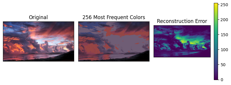
This “popularity” palette fails badly on this image. The most frequent exact colors are all clustered among the dark clouds and the dim sky, since those big regions contain many pixels with nearly the same color. The brilliant orange glow of the sunset uses many slightly different colors, each one rare, so not a single one of them makes the top 256. Those pixels get mapped to the nearest dull color in the palette, which you can see as the bright band in the error image.
Compare that to k-means, whose reconstruction is nearly indistinguishable from the original. K-means doesn’t care how often an exact color occurs, only how many pixels are near each center. So a region of many slightly different oranges still pulls a center its way. The classic median cut algorithm, used in many early GIF encoders, gets a similar benefit by recursively splitting the RGB cube into boxes holding equal numbers of pixels.