Predictive Coding

stough 202-

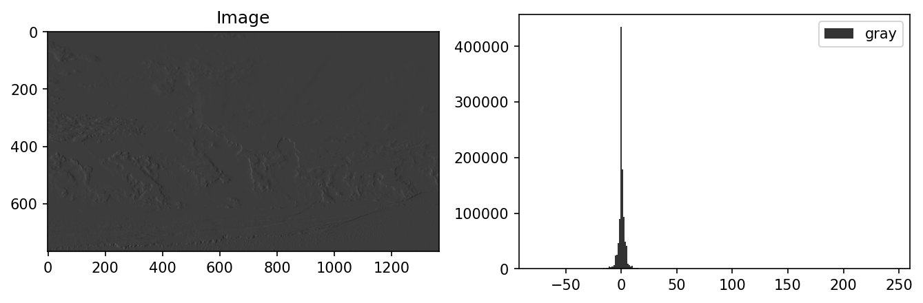
In this notebook we’re going to look at a way to account for very simple spatial redundancy, leading to much better compressibility. In short, a prediction of a pixel’s value as its left neighbor is usually pretty effective, leading to a more compressible signal than the original without any loss of information. Read on for more.

Huffman: In our discussion of entropy we noted the different kinds of redundancy that we might leverage or account for in order to compress an image. We accounted for coding redundancy by applying Huffman variable length encoding. Huffman leverages differences in the relative probability of certain pixel values over others (low entropy) to define an encoding scheme that minimizes the average number of bits needed to represent each pixel value. Huffman’s efficiency is inversely proportional to the entropy implied by the histogram of the image:

If the histogram tends toward uniform, entropy is high and Huffman coding will accomplish little.
If the histogram is highly non-uniform, with for example a few large spikes, then entropy is low and Huffman coding will work well.

Predictive coding computes some derivation of the image: the value at every pixel is its difference with respect to the pixel to the left, with the first column not changing. We’ll see that while this is a completely reversible function, such a predictive coded version of an image can be much more compressible that the original.

%matplotlib inline
import matplotlib.pyplot as plt
import numpy as np

# For spatial filtering/operations
from scipy.ndimage import (correlate,
                           convolve)
from scipy.stats import entropy

# For importing from alternative directory sources
import sys  
sys.path.insert(0, '../dip_utils')

from matrix_utils import (arr_info,
                          make_linmap)
from vis_utils import (vis_rgb_cube,
                       vis_hists,
                       vis_pair)

I = plt.imread('../dip_pics/skyandsea.jpg')
vis_hists(I)
print(arr_info(I))

((768, 1366, 3), dtype('uint8'), np.uint8(0), np.uint8(255))

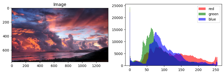
In the above, we’re viewing the image in its original, human-readable form. Let’s compute the entropy of the image.

freq, bb = np.histogram(I.ravel(), bins = np.arange(257))

entropy(freq, base=2)

np.float64(7.635605073001028)

Let’s observe just one of the color channels, without loss of generality.

J = I[...,0]
vis_hists(J)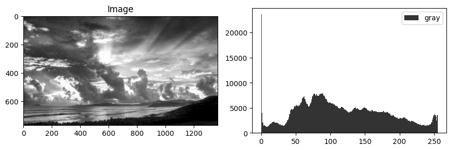

Using `correlate`¶

Here we’re going to be using the correlate method in scipy in order to apply a simple linear function to neighborhoods of pixels. This filtering is a core element of image processing from simple edge-detection to convolutional neural networks, and we will be seeing it again and again. You should read more about filtering in the spatial domain here.

In this case the neighborhood in question is extremely simple. When our process is at a pixel $i,j$ , then the neighorhood consists of that pixel and its neighbor to the left, $i,j-1$ , or 0 if the pixel is at the left edge of the image already. The linear combination of the two pixels that we want to compute is just the difference. That is,

p_{i,j}' = -1p_{i,j-1} + 1p_{i,j}

(1)

We’ll construct a simple array (also called a mask, or filter) that represents this linear combination, and then go.

h = np.array([-1, 1], ndmin=2).astype('int16')

array([[-1, 1]], dtype=int16)

arr_info(h)

((1, 2), dtype('int16'), np.int16(-1), np.int16(1))

Jf = correlate(J.astype('int16'), h, mode='constant', cval=0)
arr_info(Jf)

((768, 1366), dtype('int16'), np.int16(-76), np.int16(244))

vis_hists(Jf)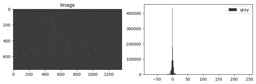

Notice that if we take one pixel (value) and subtract another pixel from it, we may get a negative number. That’s why in the above we consider the original image as int16, with both positive and negative possible values.

Look at this image and its histogram compared to the one above. Which do you think has less entropy and therefore may be more highly compressible?

I would like you to note as well that this operation is completely reversible; more on that below.

Jf[:5, :10]

array([[77, -3, -1, -3, -4, -4, -3, -4,  1, -3],
       [77, -4, -3, -4, -3, -4, -4, -2, -1, -4],
       [79, -6, -5, -3, -5, -3, -4, -2, -1, -4],
       [78, -6, -4, -5, -4, -4, -3, -3, -2, -2],
       [72, -3, -5, -5, -4, -4, -3, -3, -1, -2]], dtype=int16)

J[:5,:10]

array([[77, 74, 73, 70, 66, 62, 59, 55, 56, 53],
       [77, 73, 70, 66, 63, 59, 55, 53, 52, 48],
       [79, 73, 68, 65, 60, 57, 53, 51, 50, 46],
       [78, 72, 68, 63, 59, 55, 52, 49, 47, 45],
       [72, 69, 64, 59, 55, 51, 48, 45, 44, 42]], dtype=uint8)

Reconstructing the image is simple.¶

Considering the image Jf, the original pixels can be derived by moving from left to right, adding the numbers as you go along. The leftmost column contains original pixel values, the next column tells you how different that column is from the first. So if you simply add the first and second columns, you’ll have the original value:

\begin{split} image &= [x, y, ...] \\ \tilde{y} &= y - x \verb+ # store the difference+ \\ \tilde{y} + x &= y \verb+ # reconstruct the original+ \end{split}

This math continues to work if you just keep a running total along each row. The numpy function cumsum does exactly this for us.

Jr = np.cumsum(Jf, axis=1)
vis_hists(Jr)

freq, bins = np.histogram(J.ravel(), bins=np.arange(257))

entropy(freq, base=2)

np.float64(7.819832557813458)

Recall the original image’s entropy above, almost the entire 8 bits per pixel. What about this difference image?

ff, bb = np.histogram(Jf.ravel(), bins = np.arange(-255,257))

entropy(ff, base=2)

np.float64(3.4363483056151543)

The difference image, or predictive encoded image, has significantly less entropy. Note however that the range of possible values now is twice what is was (for any positive difference between a pixel and its left neighbor, there could be an opposite negative difference).

Further, we’ve established that the predictively encoded image has no loss of real information, in that the original can be flawlessly reconstructed.

Conclusions¶

Here we saw how predictive coding (filtering with that simple mask) is a completely reversible operation that leads to an image with significantly less entropy than the original image. Why is this?

Basically, from what we’ve learned so far, images that are interesting to us generally contain large swaths of constant or smoothly-varying color or intensity changes. That is, most of the time the context of any pixel is highly predictive of that pixel’s value itself. Where is this not the case? Really only at edges.

Since changes are smooth and small most of the time, the predictive-coded image will have many many more values close to zero, leading to a much more compressible distribution.

🧠 Further Efforts¶

We used the simplest possible predictor, the pixel to the left. Here are some ways to see how far the idea goes.

Vertical prediction. Predict each pixel from the one above it instead of the one to its left. How does the entropy compare? Does the direction of prediction matter for this image, and would it for an image with strong vertical stripes?
Guidance: Only the shape of the mask h has to change, so look at its shape with arr_info. Make sure your reconstruction with np.cumsum runs along the matching axis, and check it with np.array_equal.
Better predictors. The PNG format offers five predictors, including the average of the left and upper neighbors and the “Paeth” predictor, and picks one per row. Implement the left-and-up average. Is the entropy of its residual lower than for the left neighbor alone?
Guidance: A mask with weights on both neighbors, applied with correlate, produces the prediction error in one step. Remember that the prediction should only use pixels the decoder has already reconstructed, or it can’t be reversed. Use integer arithmetic so the result stays exactly reversible.
All three channels. Apply predictive coding to each of the R, G, and B channels of I and compare their residual entropies. Then try cross-channel prediction: predict green from red at the same pixel, and blue from green. Which works better here, predicting from a neighbor or from another channel?
Guidance: Compute the entropy of each residual with the same np.histogram and entropy calls as above. Watch the range of the residual: the difference of two uint8 values needs a signed type.
Quantize the residual. Round small differences to zero (or divide the residuals by a step size and round) before reconstructing. What happens to the entropy, and to the reconstruction? Measure the reconstruction error, and look at how it behaves as you move along a row. Why?
Guidance: Display the error image, not just a number. This one is a first step toward lossy compression, and once you can explain the behavior you find, think about how an encoder could change what it predicts from to avoid it.

Using correlate¶

Reconstructing the image is simple.¶

Conclusions¶

🧠 Further Efforts¶

Using `correlate`¶