Clustering on Color - imageprocessing-awesome

stough 202-

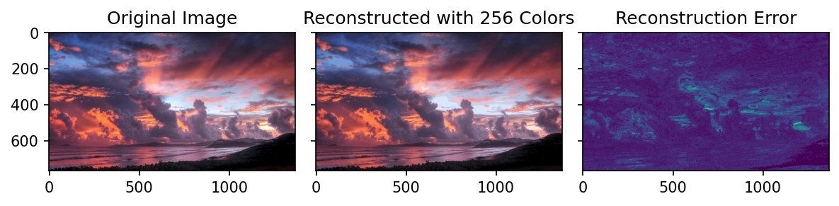
In this demo, we cluster the colors of an image using k-means clustering, leading to a selection of $K$ color centroids. Every pixel is then replaced with its centroid. This drastically reduces the number of unique colors in the image, but what happens to the quality of the image?

Why is this in a chapter on entropy and compression? A photo can easily contain over a hundred thousand distinct colors, each stored as 24 bits. If we can find a palette of just 256 representative colors, then each pixel can be stored as a single 8-bit index into that palette, cutting the size to a third before any other compression. This is indexed color, which is how GIF images and 8-bit PNGs work. It is lossy compression: the question is how to choose a palette that loses as little as possible.

Some k-means explanations...

%matplotlib inline
import scipy.cluster.vq as vq
import matplotlib.pyplot as plt
import numpy as np

# For importing from alternative directory sources
import sys  
sys.path.insert(0, '../dip_utils')

from matrix_utils import arr_info
from vis_utils import (vis_rgb_cube,
                       vis_image,
                       vis_triple,
                       vis_hists,
                       vis_pair)

COLORS = 256

I = plt.imread('../dip_pics/skyandsea.jpg')
arr_info(I)

((768, 1366, 3), dtype('uint8'), np.uint8(0), np.uint8(255))

vis_image(I, title='Original Image')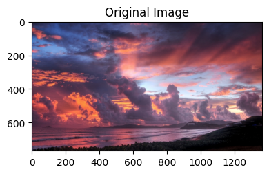

Now we’ll consider the image as a collection of R,G,B points¶

X = np.concatenate([np.expand_dims(IC, axis = 1) for IC in
                    [I[...,0].ravel(), I[...,1].ravel(), I[...,2].ravel()]], axis = 1)
#X is N*Mx3

#Needs floating point data to work with, we'll translate back.
Xf = X.copy().astype('float')

# Xf = vq.whiten(Xf)
# The kmeans documentation asks for this, but results seem easier to deal with
# if I don't use it.

arr_info(Xf)

((1049088, 3), dtype('float64'), np.float64(0.0), np.float64(255.0))

Use scipy’s vector quantization module to perform K-Means on the data¶

K-means looks for $K$ cluster centers such that every point is close to its nearest center. It alternates two steps: assign every point (here, every pixel’s RGB color) to its nearest center, then move each center to the mean of the points assigned to it. Repeat until things stop changing. Each final center is the average of a group of similar colors, so the centers make a natural palette: there will be many centers among the colors the image uses a lot, and few where it uses little.

#Ask kmeans to get us 256 colors.
[centers, labels] = vq.kmeans2(Xf, COLORS)
centersUint = centers.copy().astype('uint8')
# uint8 versions of the centers will clip to 0-255 for us, just in case.

# Why do some centers end up outside of [0, 255]? I tried to include all the centers,
# but then the colors associated with labels warp toward gray, kind of washing out
# the image...SO don't do this
# centerscopy = centers.copy()
# centerscopy = centerscopy - centerscopy.min()
# centerscopy = centerscopy/centerscopy.max()
# centersUint = np.array(255*centerscopy).astype('uint8')

/tmp/ipykernel_3069/1288621509.py:2: UserWarning: One of the clusters is empty. Re-run kmeans with a different initialization.
  [centers, labels] = vq.kmeans2(Xf, COLORS)

# Explore centers, labels.
print(arr_info(centers))
print(arr_info(labels))

((256, 3), dtype('float64'), np.float64(-89.13305913225767), np.float64(301.86181576930903))
((1049088,), dtype('int32'), np.int32(0), np.int32(255))

Note that the above k-means gives us back the COLORS number of centroids called centers, each of which is an RGB point, as well as a labels array that indexes this centers for each pixel in the original image. We also cast to uint8 to ensure valid colors (RGB each in [0,255]).

About the comment in the k-means cell above, wondering why some centers land outside $[0,255]$ : by default kmeans2 starts from random centers drawn from a Gaussian fit to the data, and a Gaussian can easily produce values outside the valid color range. If such a center starts far from all the data, no pixel ever gets assigned to it. It becomes an empty cluster and never moves (kmeans2 warns about this). These unused centers are why the reconstructed image ends up with somewhat fewer than COLORS distinct colors, as we’ll count below. Casting to uint8 is harmless for them, since no pixel uses them.

labels[:10]

array([115, 115, 79, 105, 105, 105, 207, 228, 207, 207], dtype=int32)

centersUint[labels[:10]]

array([[79, 43, 61],
       [79, 43, 61],
       [72, 44, 64],
       [66, 40, 59],
       [66, 40, 59],
       [66, 40, 59],
       [56, 44, 61],
       [54, 39, 57],
       [56, 44, 61],
       [56, 44, 61]], dtype=uint8)

Here we’ll create a new image, where every pixel in the original is replace with the centroid color it is closest to.¶

#centers is 256x3 representative colors from the image, while
#labels is I.size indexes that tells which row of centers best
#represents (is closest to) each and every pixel of the image.

#Now, make an image consisting of the colors that each pixel got mapped to.
Ir = centersUint[labels].reshape(I.shape)

# Alternative way to do the same thing, each channel separately:
# Ir = np.zeros(I.shape)
# Ir[...,0] = np.reshape(centersUint[labels, 0], I.shape[:2])
# Ir[...,1] = np.reshape(centersUint[labels, 1], I.shape[:2])
# Ir[...,2] = np.reshape(centersUint[labels, 2], I.shape[:2])

#Somehow, Ir is still floating point, so the imshow colormap will be weird.
#We'll just cast it to uint8
# Ir = Ir.astype('uint8')

In the above we sample the centersUint of color centroids for every pixel in the original image, and we reshape the resulting H*W x 3 to a H x W x 3.

#Get and display an error image. We'll use scipy.cluster.vq
#https://docs.scipy.org/doc/scipy/reference/generated/scipy.cluster.vq.vq.html
color_codes, dist = vq.vq(Xf, centersUint)

vis_triple(I, Ir, np.reshape(dist, I.shape[:2]),
           first_title='Original Image',
           second_title='Reconstructed with %d Colors' % COLORS,
           third_title='Reconstruction Error')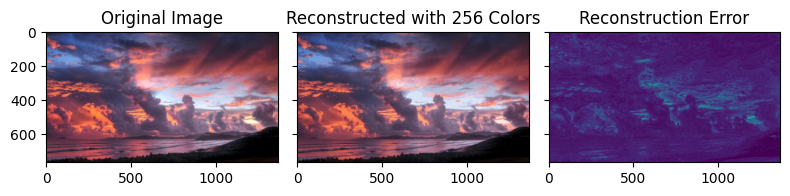

#And just to prove it, look at unique.
#with numpy 1.13, you can send an axis to unique.
#https://stackoverflow.com/questions/16970982/find-unique-rows-in-numpy-array
#But I'll write it more generally.
origvals = I[...,0].astype('uint32').ravel() \
      + 256*I[...,1].astype('uint32').ravel() \
      + 256**2*I[...,2].astype('uint32').ravel()
newvals = Ir[...,0].astype('uint32').ravel() \
      + 256*Ir[...,1].astype('uint32').ravel() \
      + 256**2*Ir[...,2].astype('uint32').ravel()

print('Original image has %d unique colors, versus %d in the cluster-colored image.' %
      (len(np.unique(origvals)), len(np.unique(newvals))))

# By the way, AI notes a simpler way to do this:
# rgb_view = I.reshape(-1, 3).view(np.uint32)
# num_unique = len(np.unique(rgb_view))

Original image has 124085 unique colors, versus 230 in the cluster-colored image.

How Much Did We Save?¶

The original pixels take 24 bits each. The palette version takes 8 bits per pixel (an index into centersUint), plus a negligible $256 \times 3$ bytes for the palette itself. And the indices are themselves a signal with an entropy, so we can ask how many bits per pixel a Huffman code of the labels would need:

from scipy.stats import entropy

H_labels = entropy(np.bincount(labels, minlength=COLORS), base=2)
print(f'original:          24 bits/pixel')
print(f'palette indices:    8 bits/pixel')
print(f'entropy of labels: {H_labels:.2f} bits/pixel')
print(f'compression ratio, Huffman-coded labels: about {24/H_labels:.1f}')

original:          24 bits/pixel
palette indices:    8 bits/pixel
entropy of labels: 7.55 bits/pixel
compression ratio, Huffman-coded labels: about 3.2

The labels are spread pretty evenly over the palette, which is exactly what k-means aims for, so their entropy is only a little under 8 bits. Most of the savings come from the palette itself. To do much better we’d need to also exploit spatial redundancy, the fact that neighboring pixels usually share a label, which is where predictive coding comes in.

Viewing the Color Cubes¶

vis_rgb_cube(I)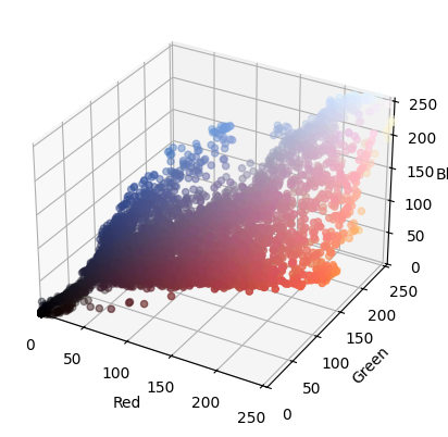

Before viewing the RGB color cube of the clustered reconstruction, think about what you would expect it to look like given the above color cube of the original image.¶

vis_rgb_cube(Ir)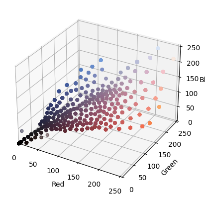

🧠 Further Efforts¶

Try out for yourself some of the following.

How many colors do you need? Change COLORS (try 4, 16, 64, and 256) and compare the reconstructed images. At what point does the image look “right” to you?
Guidance: Rather than re-running the notebook by hand, write a loop that clusters with several values of $K$ and shows the reconstructions together. $K$ -means on every pixel of this image is slow, so fit the clusters to a random sample of pixels (as in the matplotlib tutorial) and then assign every pixel with vq.vq.
Measure the reconstruction error. Recall the cell including color_codes, dist = vq.vq(Xf, centersUint) that gives the error, or fidelity loss, at every pixel. Plot the average error against $K$ . Where is the “elbow”, beyond which more colors buy little improvement?
Guidance: Use the same pixel sample for every $K$ so the comparison is fair. Plot $K$ on a log axis.
Where do the colors go? Use np.bincount(labels) to find which palette colors are used most, and show the palette sorted by how many pixels use each color. Before you look, predict which parts of the image will get many palette colors and which will get few.
Guidance: A palette is easy to display as a $1 \times K$ (or $16 \times 16$ ) image of the centers. Compare with where the reconstruction error is largest.
Different images. Cluster a different image: a cartoon or logo, a photo with large smooth regions, a busy natural scene. Which can get by with a small palette, and why? What kind of images are amenable to smaller color dictionaries without too much fidelity loss?
Guidance: Think about the color cubes: how many separate clumps of points does each image have?
Other ways to choose a palette. The median cut algorithm, used by many GIF encoders, repeatedly splits the color cube at the median of its widest channel. Implement it, or use Pillow’s Image.quantize, and compare it with k-means at the same $K$ , in error and in speed.
Guidance: Compare at the same $K$ with the same error measure as above, so the comparison is fair.