K-means single iteration - imageprocessing-awesome

stough 202-

Demo on k means clustering. We generate a little data and then do a single step of the EM scheme for clustering.

Finding objects in images:

Color coherence
Spatial coherence

Pixels belonging to the same object tend to have similar colors (color coherence) and to be near one another (spatial coherence). Clustering groups data points that are similar, so it’s a natural first step toward finding objects. K-means is the simplest and most widely used clustering method. Given a number of clusters $K$ , it looks for $K$ cluster centers $\mathbf{c}_1, \ldots, \mathbf{c}_K$ and an assignment of every point to a cluster that minimize the total squared distance from each point to its center:

J = \sum_{i=1}^{N} \left\| \mathbf{x}_i - \mathbf{c}_{k(i)} \right\|^2

where $k(i)$ is the cluster point $i$ is assigned to. We’ll first see the algorithm on easy 2D data, then on the colors of an image, and finally in SLIC superpixels, which clusters on color and position.

%matplotlib inline
import matplotlib.pyplot as plt
import numpy as np
from numpy import random

# For importing from alternative directory sources
import sys  
sys.path.insert(0, '../dip_utils')

from matrix_utils import (arr_info,
                          make_linmap)
from vis_utils import (vis_rgb_cube,
                       vis_hists,
                       vis_pair,
                       vis_surface)

from scipy.spatial.distance import cdist

K = 2
NUMPOINTS = 1000

# Let's generate 2d random data
X1 = np.random.randn(NUMPOINTS//2, 2)  # Unit normal (mean 0, var 1)
X2 = np.random.randn(NUMPOINTS//2, 2)

X2[:,0] = 5 + 2*X2[:,0]
X2[:,1] = 3 + 2*X2[:,1]  # X2 data should be mean (5,3) var 4

X = np.concatenate([X1, X2], axis=0)

Two blobs of 500 points each: one centered at $(0,0)$ with variance 1, and one centered at $(5,3)$ with variance 4, so it’s more spread out. We know the right answer here, which makes it easy to see how k-means does.

Look at the generated data¶

plt.figure()
plt.scatter(X[:,0], X[:,1])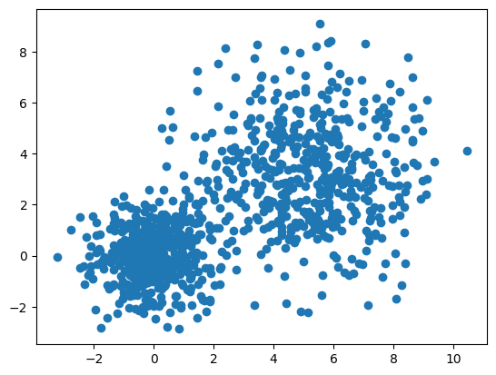

# For fun: Let's pick some random (and good) cluster colors
clusterColors = np.random.rand(K, 3) # Picking random colors for each cluster.
varsSoFar = np.var(clusterColors, axis=0) # Should be 1 x 2 of the variance of each column.

for i in range(3*K):
    tempColors = random.rand(K, 3) #Picking K random colors
    vartemp = np.var(tempColors, axis=0)
    if np.all(vartemp > varsSoFar):
        clusterColors = tempColors
        varsSoFar = vartemp

Step 0: initialize¶

K-means needs a starting guess for the centers. A simple choice is $K$ distinct data points picked at random.

# K-means: initialization
# pick K initial cluster centers.
# whichinit = random.randint(0, len(X), size=(K,)) # Could generate repeats.
whichinit = random.choice(len(X), size=K, replace=False)
CC = X[whichinit, :].copy() # Cluster Centers

CC_init = CC.copy()

CC

array([[4.67585676, 4.24890125],
       [1.946762  , 4.81379048]])

plt.figure(figsize=(4,4))
plt.scatter(X[:,0], X[:,1], c='gray', alpha=.5)
plt.scatter(CC[:,0], CC[:,1], s=30, c=clusterColors)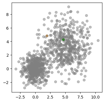

Step 1: assign each point to its nearest center¶

cdist computes the distance from every point (row of X) to every center (row of CC), an $N \times K$ matrix. argmin along each row then picks the closest center for each point. With the centers fixed, this is the assignment that makes $J$ as small as possible.

# K-means: compute: for every data point determine which center is closest.
# Need some magic function that computes the distance between every row of X
# (the points) and every row of CC (the clusters).
D = cdist(X, CC, 'euclidean')
# D should be NUMPOINTS x K

whichCluster = np.argmin(D, axis=1) # NUMPOINTS x 1 of which center was closest

D[:10,:]

array([[5.52699637, 4.5086391 ],
       [6.41080128, 5.09573214],
       [4.54117375, 4.18543854],
       [5.15470562, 4.14259554],
       [7.35665814, 6.3058581 ],
       [6.42398001, 5.24878489],
       [5.83518661, 4.44120574],
       [5.80056776, 4.33449988],
       [6.40652037, 5.32732835],
       [6.83636001, 5.85796149]])

X[0,:]

array([0.60634515, 0.50901299])

plt.figure(figsize=(4,4))
plt.scatter(X[:,0], X[:,1], c=clusterColors[whichCluster], alpha=.5)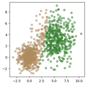

With only two centers, the boundary between the clusters is a straight line, the perpendicular bisector between the two centers. Points on either side go to the nearer center, whether or not that matches the true blobs.

Step 2: move each center to the mean of its points¶

Now hold the assignments fixed, and ask where each center should be to make $J$ as small as possible. The point that minimizes the total squared distance to a set of points is their mean, so each center moves to the average of the points assigned to it.

# K-means: recompute the cluster centers as the mean of the data in each cluster
for c in range(K):
    CC[c,:] = np.mean(X[whichCluster == c, :], axis=0) # average of just those that were closest to c.

np.mean(X[whichCluster == 0, :],axis=0)

array([5.63446637, 3.09083537])

(whichCluster == 1).sum()

np.int64(579)

plt.figure(figsize=(4,4))
plt.scatter(X[:,0], X[:,1], c='gray', alpha=.5)
plt.scatter(CC[:,0], CC[:,1], s=30, c=clusterColors)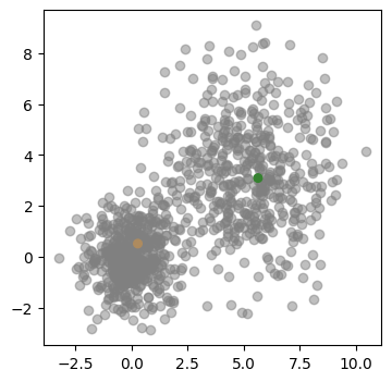

Repeat¶

That’s one iteration: assign, then update. Now we assign again using the moved centers, then update again, and so on. Each step can only lower $J$ (or leave it unchanged), and there are only finitely many ways to assign the points, so the process must eventually stop changing: k-means always converges. Here’s the second assignment:

# K-means: compute: for every data point determine which center is closest.
# Need some magic function that computes the distance between every row of X
# (the points) and every row of CC (the clusters).
D = cdist(X, CC, 'euclidean')
# D should be NUMPOINTS x K

whichCluster = np.argmin(D, axis=1) # NUMPOINTS x 1 of which center was closest

plt.figure(figsize=(4,4))
plt.scatter(X[:,0], X[:,1], c=clusterColors[whichCluster], alpha=.5)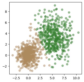

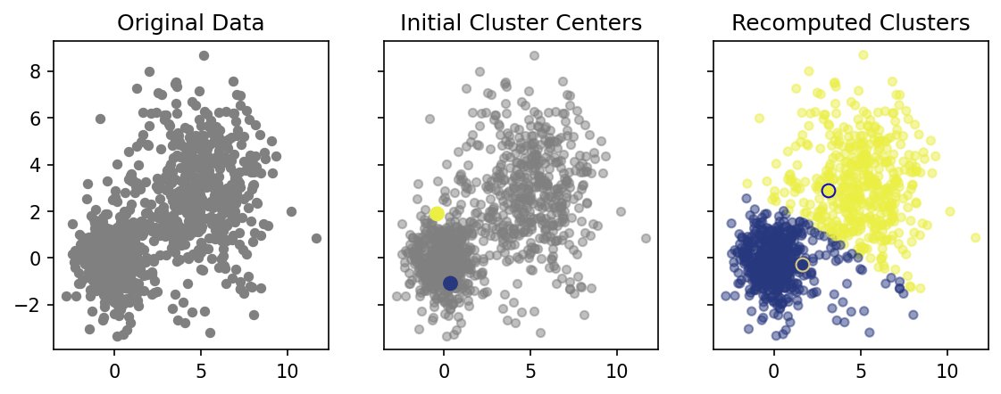
A summary of the first iteration: the data, the random initial centers, and the clusters and centers after one update.

f, ax = plt.subplots(1,3, figsize=(9,3), sharex=True, sharey=True)
ax[0].scatter(X[:,0], X[:,1], c='gray', s=20)
ax[0].set_title('Original Data')


ax[1].scatter(X[:,0], X[:,1], c='gray', alpha=.5, s=20)
ax[1].scatter(CC_init[:,0], CC_init[:,1], c=clusterColors, s=50)
ax[1].set_title('Initial Cluster Centers')






pointColors = clusterColors[whichCluster]
clusterEdgeColors = 1 - clusterColors # for contrast, make the cluster center edges opposite.

ax[2].scatter(X[:,0], X[:,1], c=pointColors, alpha=.5, s=20)
ax[2].scatter(CC[:,0], CC[:,1], c=clusterColors, edgecolors=clusterEdgeColors, s=50)
ax[2].set_title('Recomputed Clusters')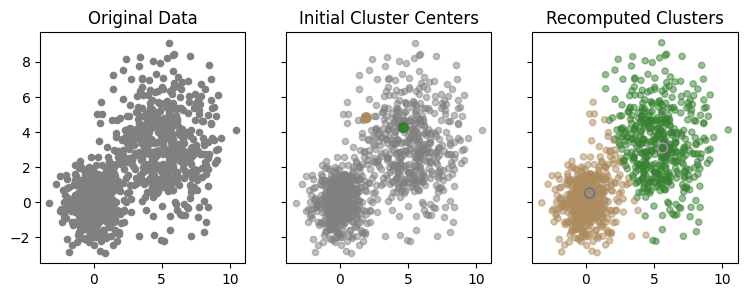

Running to convergence¶

In practice we just loop until the assignments stop changing. This is the EM-style alternation in a few lines, starting again from the same initial centers:

CC = CC_init.copy()
assignments = None
for it in range(100):
    newAssignments = np.argmin(cdist(X, CC), axis=1)          # step 1: assign
    if assignments is not None and np.all(newAssignments == assignments):
        break
    assignments = newAssignments
    CC = np.stack([X[assignments == c].mean(axis=0) for c in range(K)])  # step 2: update
    J = np.sum((X - CC[assignments])**2)
    print(f'iteration {it}: J = {J:9.1f}, centers = {CC.round(2).tolist()}')

plt.figure(figsize=(4,4))
plt.scatter(X[:,0], X[:,1], c=clusterColors[assignments], alpha=.5, s=20)
plt.scatter(CC[:,0], CC[:,1], c=clusterColors, edgecolors='k', s=80)
plt.title(f'Converged after {it} iterations');

iteration 0: J =    5436.5, centers = [[5.63, 3.09], [0.28, 0.52]]
iteration 1: J =    4540.1, centers = [[5.43, 3.37], [0.14, 0.14]]
iteration 2: J =    4509.8, centers = [[5.36, 3.39], [0.13, 0.07]]
iteration 3: J =    4508.4, centers = [[5.34, 3.38], [0.11, 0.06]]
iteration 4: J =    4508.3, centers = [[5.33, 3.39], [0.11, 0.05]]

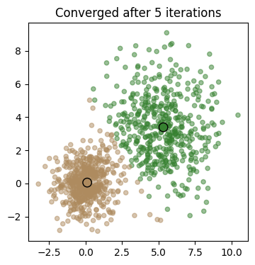
$J$ decreases at every iteration, and within a handful of iterations the centers settle near the true blob centers, $(0,0)$ and $(5,3)$ . They won’t be exactly there, though. K-means draws the boundary halfway between centers, so the wide blob’s outlying points that fall closer to the tight blob’s center get assigned to it, pulling that center slightly toward the wide blob. Losing those points pushes the wide blob’s center slightly away. K-means implicitly assumes round clusters of similar size.

Two other caveats to keep in mind:

Initialization matters. K-means finds a local minimum of $J$ , not necessarily the best one. Re-run the notebook a few times: on easy data like this it nearly always finds the same answer, but on harder data different starting centers can give different clusterings. Practical implementations run several random starts and keep the best, or use smarter seeding such as k-means++.
You have to choose $K$ . Try K = 3 at the top. K-means will happily split the data into three clusters whether or not three is meaningful.