K-means iteration - imageprocessing-awesome

stough 202-

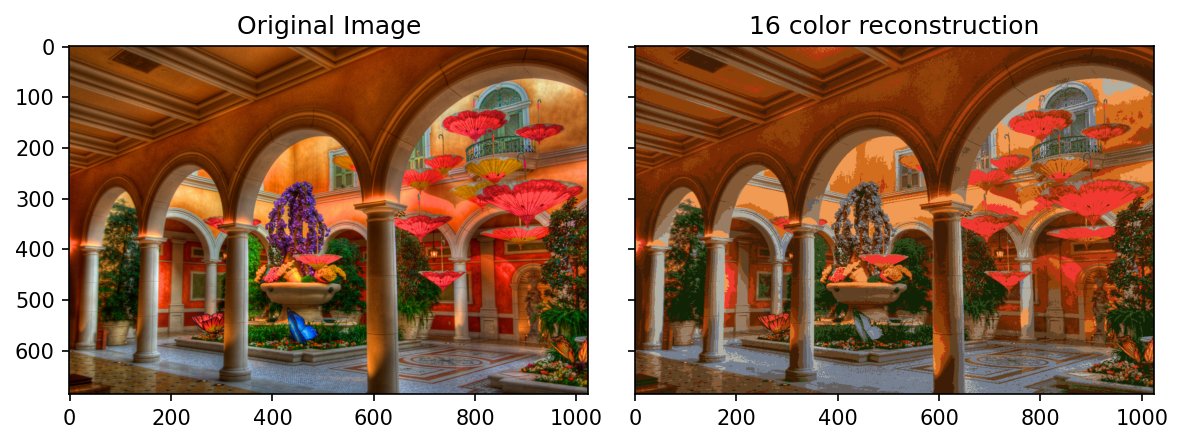
Here we do k-means clustering on an image, to get representative colors for the image.

This is the same k-means algorithm as on the 2D toy data, applied to real data: every pixel becomes a point in 3D RGB space, and we look for $K=16$ cluster centers among them. The centers become a 16-color palette, and replacing every pixel by its center’s color gives a 16-color version of the image. It’s the same idea as the color clustering we did for compression, except that here we write the k-means loop ourselves instead of calling scipy.

%matplotlib inline
import matplotlib.pyplot as plt
import numpy as np

# For importing from alternative directory sources
import sys  
sys.path.insert(0, '../dip_utils')

from matrix_utils import (arr_info,
                          make_linmap)
from vis_utils import (vis_rgb_cube,
                       vis_hists,
                       vis_pair,
                       vis_surface)

from scipy.spatial.distance import cdist

K = 16
MAXITER = 20
NUMPOINTS = 100

I = plt.imread('../dip_pics/bellagio.jpg').astype(float)
X = np.stack([I[...,i].ravel() for i in range(3)]).T

X has one row per pixel, its $(R, G, B)$ values: $687 \cdot 1024 \approx 700{,}000$ points in 3D. The position of each pixel is thrown away; k-means here only sees colors.

plt.figure()
plt.imshow(I/255)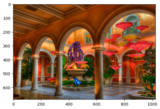

X[:10,:]

array([[118.,  57.,   0.],
       [117.,  55.,   8.],
       [125.,  64.,  10.],
       [130.,  70.,   8.],
       [119.,  58.,   3.],
       [118.,  57.,  10.],
       [112.,  52.,   2.],
       [115.,  57.,  11.],
       [104.,  52.,   4.],
       [126.,  61.,   7.]])

# For fun: Let's pick some random (and good) cluster colors
clusterColors = np.random.rand(K, 3) # Picking random colors for each cluster.
varsSoFar = np.var(clusterColors, axis=0) # Should be 1 x 2 of the variance of each column.

for i in range(3*K):
    tempColors = np.random.rand(K, 3) #Picking K random colors
    vartemp = np.var(tempColors, axis=0)
    if np.all(vartemp > varsSoFar):
        clusterColors = tempColors
        varsSoFar = vartemp

clusterColors

array([[0.76003431, 0.56815207, 0.9851263 ],
       [0.85421562, 0.25820378, 0.30594259],
       [0.65376703, 0.44425113, 0.13264375],
       [0.95164059, 0.4366015 , 0.51904003],
       [0.10403741, 0.80160196, 0.68704969],
       [0.53130825, 0.79647325, 0.11111253],
       [0.62247207, 0.93161496, 0.90251527],
       [0.98172557, 0.92461134, 0.34947592],
       [0.71629537, 0.04163917, 0.93777949],
       [0.33731721, 0.50553171, 0.84051477],
       [0.35672791, 0.52013192, 0.60819852],
       [0.98595808, 0.04073001, 0.44196889],
       [0.98060839, 0.29174707, 0.24579029],
       [0.43551398, 0.88727809, 0.05929939],
       [0.37075392, 0.06199934, 0.97468878],
       [0.17794268, 0.17501959, 0.23886008]])

Pick some initial cluster centers.¶

# K-means: initialization
# pick K initial cluster centers.
# whichinit = random.randint(0, len(X), size=(K,)) # Could generate repeats.
whichinit = np.random.choice(len(X), size=K, replace=False)
CC = X[whichinit, :].copy() # Cluster Centers

As before, we start from $K$ randomly chosen pixels. Since every pixel is equally likely to be picked, the initial centers tend to come from the colors that cover the most area. In this image those are the warm reds, oranges, and browns.

CC_init = CC.copy()
CC

array([[149.,  62.,   9.],
       [ 87.,  37.,   0.],
       [ 97.,  45.,   5.],
       [122.,  59.,   6.],
       [ 92.,  48.,   0.],
       [ 78.,  65.,  20.],
       [ 67.,  56.,  36.],
       [100.,  55.,  26.],
       [ 97.,  48.,  15.],
       [113.,  61.,  22.],
       [119.,  51.,  14.],
       [ 96., 112., 127.],
       [  2., 120., 226.],
       [152.,  66.,   5.],
       [154., 117.,  65.],
       [143., 101.,  63.]])

The main Expectation-Maximization loop¶

Basically, we assign a cluster to each point, and then recompute the clusters based on that assignment.

Each pass computes all $700{,}000 \times 16$ pixel-to-center distances, which is why this takes a few seconds. We run a fixed MAXITER iterations rather than checking for convergence. The if np.any(...) guard skips any center that ends up with no pixels (an empty cluster), which would otherwise give an undefined mean.

# K-means: compute: for every data point determine which center is closest.
# Need some magic function that computes the distance between every row of X
# (the points) and every row of CC (the clusters).
for i in range(MAXITER):
    D = cdist(X, CC, 'euclidean')
    # D should be NUMPOINTS x K

    whichCluster = np.argmin(D, axis=1) # NUMPOINTS x 1 of which center was closest

    # K-means: recompute the cluster centers as the mean of the data in each cluster
    for c in range(K):
        if np.any(whichCluster == c):
            CC[c,:] = np.mean(X[whichCluster == c, :], axis=0) # average of just those that were closest to c.

# Doing this on a big image, don't want to scatter 100Ks of points, really slow.
rands = np.sort(np.random.choice(len(X), size=500*K, replace=False))


f, ax = plt.subplots(1,3, figsize=(9,3), sharex=True, sharey=True)
ax[0].scatter(X[rands,0], X[rands,1], c='gray', s=20)
ax[0].set_title('Original Data')


ax[1].scatter(X[rands,0], X[rands,1], c='gray', alpha=.5, s=20)
ax[1].scatter(CC_init[:,0], CC_init[:,1], c=CC_init/255, s=50)
ax[1].set_title('Initial Cluster Centers')


pointColors = CC[whichCluster[rands], :]
clusterEdgeColors = 1 - clusterColors # for contrast, make the cluster center edges opposite.
# clusterEdgeColors = 1 - CC/255 # for contrast, make the cluster center edges opposite.

ax[2].scatter(X[rands,0], X[rands,1], c=pointColors/255, alpha=.5, s=20)
ax[2].scatter(CC[:,0], CC[:,1], c=CC/255, edgecolors=clusterEdgeColors, s=50)
ax[2].set_title('Recomputed Clusters')

plt.tight_layout()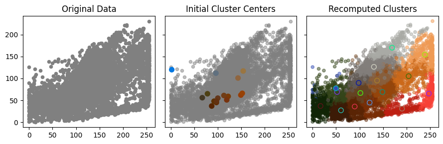

We can’t easily draw 700,000 points, so these scatters show a random sample, and only two of the three dimensions: red on the x-axis, green on the y-axis (blue is hidden). On the right, each sampled pixel is drawn in the color of its cluster center, and the centers are circled. The centers spread out to cover the cloud of colors, with more of them where the data is dense.

f, ax = plt.subplots(1,2, figsize=(8,3), sharex=True, sharey=True)

ax[0].imshow(I/255)
ax[0].set_title('Original Image')

# Reconstructed Image.
Ir = np.reshape(CC[whichCluster,:], I.shape)
ax[1].imshow(Ir/255) # Because it's floating point.
ax[1].set_title('{} color reconstruction'.format(K))

plt.tight_layout()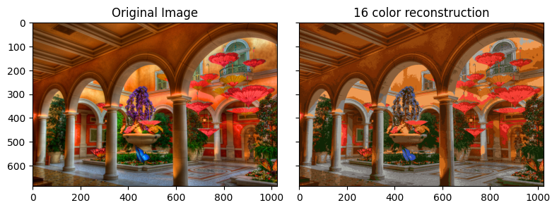

Sixteen colors capture the warm architecture remarkably well. But look at the purple flowers and the blue accents in the middle: they’ve lost their color, mapped to a nearby gray or brown. They cover so few pixels that they don’t pull a center of their own. K-means minimizes total squared error, so it spends its 16 colors where most of the pixels are. Try increasing K, and watch when the purple comes back.

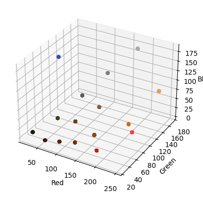
The color cubes below show the same thing in 3D: the original’s continuous cloud of colors collapses to just 16 points.

vis_rgb_cube(I)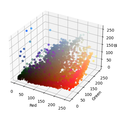

vis_rgb_cube(Ir)