SLIC Superpixels

stough, 202-

DIP 10.5

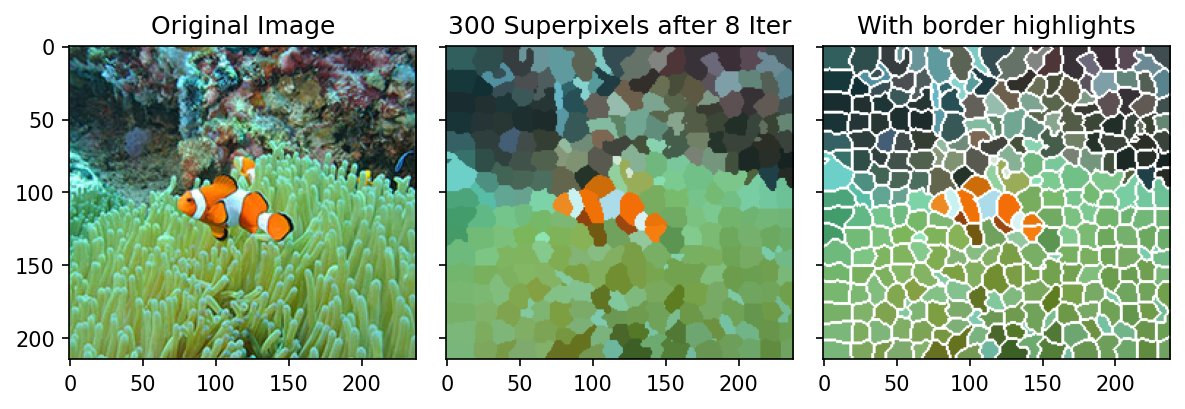
This shows Simple Linear Iterative Clustering at work to show superpixel segmentation of images. We’ll split this up to look at the algorithm in detail. skimage includes numerous segmentation methods, but we’re interested here in understanding the details.

Superpixels are small, compact regions of similar color: an over-segmentation of an image into a few hundred pieces that respect its edges. Working with 300 superpixels instead of 300,000 pixels makes many later steps, like segmentation, object detection, and labeling, much cheaper, while losing little, since pixels within a superpixel are nearly alike anyway.

SLIC (Achanta et al., 2012) is k-means with two twists:

Each pixel is a point in a 5D space: its three color values and its two spatial coordinates. Clustering on color alone (as in our image k-means demo) groups same-colored pixels from anywhere in the image. Adding position makes the clusters spatially compact.
Each cluster center only searches a local window around itself, $2S \times 2S$ pixels where $S$ is the grid spacing. Standard k-means compares every pixel against every center, $O(NK)$ work per iteration. SLIC compares each pixel against only the few centers whose windows overlap it, so the cost is $O(N)$ no matter how many superpixels we ask for.

Below we build it up step by step.

Parameters¶

SUPERPIXELS is roughly how many superpixels we want. MAXITER and T control when the iterations stop: after MAXITER iterations, or once the cluster centers move less than T in total.

%matplotlib inline
import matplotlib.pyplot as plt
import numpy as np
from scipy.spatial.distance import cdist
import scipy.stats as stats
import scipy.ndimage as ndimage

import skimage.filters as filters
import skimage.color as color


IMAGE = 'clown_fish.jpg'
# IMAGE = 'bellagio.jpg'

SUPERPIXELS = 300
MAXITER = 20
T = 10 # convergence threshold.

Helper functions¶

myfunc returns the most common label in a neighborhood. We’ll use it at the end to clean up stray pixels.

#clean-up function for the label image.
def myfunc(x):
    return stats.mode(x, axis=None)[0]

reinitM nudges each initial center to the lowest-gradient pixel in its $3 \times 3$ neighborhood. A center that happens to land exactly on an edge, or on a noisy pixel, would start with an unrepresentative color. Moving it to the flattest nearby spot avoids that. (The gradient magnitude comes from the Sobel filter.)

def reinitM():
    global M, I, s, ishape

    # Should pick the lowest gradient pixel among neighbors of each cluster
    # to reinitialize it. So, get gradient image.
    gradI = filters.sobel(color.rgb2gray(I))

    # Now, loop over each cluster and see if we should move it slightly.
    for mi in range(len(M)):
        i, j = [int(q) for q in np.round(M[mi, 3:])]
        curbest = gradI[i,j] # minimum gradient so far.
        bi, bj = i, j # best i and j so far.

        # look over all our immediate neighbors for lowest gradient.
        for x in range(i-1, i+2):
            if x < 0 or x >= I.shape[0]:
                continue
            for y in range(j-1, j+2):
                if y < 0 or y >= I.shape[1]:
                    continue

                if gradI[x,y] < curbest:
                    curbest = gradI[x,y]
                    bi, bj = x, y

        M[mi, :] = np.concatenate((I[bi, bj], [bi, bj]), axis=0)

convergedYet measures how far all the cluster centers moved during the last iteration, and reports convergence once that total is below T.

def convergedYet():
    global M, Mprev, iteration
    normdiff = np.sqrt(np.sum((M-Mprev)**2))
    print('iteration %d normdiff %f.' % (iteration, normdiff))
    return normdiff < T

Load the image, and choose the grid spacing and the color/space trade-off¶

With $N$ pixels and $K$ superpixels, each superpixel should cover about $N/K$ pixels, so the grid spacing is $S = \sqrt{N/K}$ (s in the code).

SLIC’s distance between a pixel and a cluster center combines color distance $d_c$ and spatial distance $d_s$ (Eq. 10-91 in DIP):

D = \sqrt{d_c^2 + \left(\frac{d_s}{S}\right)^2 m^2}

Dividing $d_s$ by $S$ puts distance in units of “grid spacings”. The compactness $m$ (here cs $= m^2$ ) sets the trade-off. Large $m$ makes spatial distance dominate, giving regular, nearly square superpixels that ignore edges. Small $m$ lets color dominate, so superpixels follow edges closely but get irregular shapes. Try changing cs and see.

(One difference from the paper: we measure color distance in RGB. Achanta et al. use CIELAB, where Euclidean distance better matches perceived color difference.)

I = plt.imread('../dip_pics/' + IMAGE).astype('float')
ishape = I.shape

# s = the sampling interval.
s = int(np.round(np.sqrt((ishape[0]*ishape[1])//SUPERPIXELS)))

# cs = the color distance scaler square, see Eq. 10-91
# cs = 3*255**2 #Just the maximum color discrepancy: weights regular regions highly.
cs = 100**2 # Trying for image boundaries instead of spatial regularity.

Initialize the cluster centers¶

We place the centers on a regular grid every s pixels. Each row of M is one center: $[R, G, B, row, col]$ , its color and position. Then reinitM nudges each one off of any edge.

# Make M, the initial cluster centers. This should be SUPERPIXELS x 5, for
# the spatial coords of the cluster centers and the average color of them.
M = np.concatenate([np.expand_dims(IC, axis=1) for IC in
                    [I[s::s, s::s, 0].ravel(),
                     I[s::s, s::s, 1].ravel(),
                     I[s::s, s::s, 2].ravel(),
                     ]], axis=1)
xm = np.meshgrid(np.arange(s, ishape[0], s), np.arange(s, ishape[1], s), indexing='ij')
M = np.append(M, np.concatenate([np.expand_dims(xi, axis=1) for xi in
                                 [x.ravel() for x in xm]], axis=1),
              axis=1)


# Here we should reinitialize these M to the lowest-gradient point in the 3x3,
# but we won't yet.
reinitM()

# Maintain a copy of the previous M, so that we can tell if it is converging.
Mprev = M.copy()

Precompute¶

D holds, for every pixel, the distance to the best center found so far, and L holds that center’s label. Both get reset as better centers are found. Since every center searches a window of the same size, the spatial distance from the window’s center to each of its pixels is the same every time. We compute it once, as spaceDist.

# Initial distance measure D for every pixel, and label
# D = np.finfo.max*np.ones((ishape[0], ishape[1]))
D = 1.0e20*np.ones((ishape[0], ishape[1]))
L = -1*np.ones((ishape[0], ishape[1]))


# Eq. 10-91 shows that the distance we want is a combination of the
# spatial and color distance. The spatial distance doesn't change though,
# in that i+x, j+y is always a fixed distance from i,j. We should precompute
# all of those distances...but not now.


# The spatial distance is constant over all windows [-s, s] for every
# cluster, so we'll just precompute. We'll also get the coordinate of the
# whole window in xr, yr, for use later as well.
xr, yr = np.meshgrid(np.arange(-s, s + 1), np.arange(-s, s + 1), indexing='ij')
scoords = np.concatenate([np.expand_dims(x, axis=1) for x in [xr.ravel(), yr.ravel()]], axis=1)
sDist = np.sqrt(np.sum(scoords**2, axis = 1))
spaceDist = np.reshape(sDist, (2*s+1, 2*s+1)) # distance from origin of the window, as matrix.



# xs are the x and y coords of every pixel. used for average computing later.
xs = np.meshgrid(np.arange(ishape[0]), np.arange(ishape[1]), indexing='ij')

The main loop: assign, then update¶

This is k-means, with the local-window twist:

Assign: for each center, look at every pixel in the $(2S+1) \times (2S+1)$ window around it, and compute the combined distance $D$ . Wherever that’s smaller than the pixel’s current best distance, claim the pixel for this center. (The commented-out double for-loop is the straightforward version. The numpy version does the same thing for the whole window at once, which is much faster.)
Update: move each center to the mean color and mean position of the pixels it claimed.
Stop when the centers barely move.

iteration = 0

while True:
    # First, loop over clusters and assign pixels to them.
    for mi, mx in enumerate(M):
        # mi is 1x5 of the average color and position of the cluster.
        i, j = [int(q) for q in np.round(mx[3:5])]
        # look over all pixels in the 2s x 2s neighborhood to see if they belong
        # to this cluster.

        # This is the double for-loop in python, exhaustive scheme.
        # for x in range(i - s, i + s + 1):
        #     if x < 0 or x >= ishape[0]:
        #         continue
        #
        #     for y in range(j - s, j + s + 1):
        #         if y < 0 or y >= ishape[1]:
        #             continue
        #
        #         sDist = np.sqrt((x-i)**2 + (y-j)**2)
        #         cxy = I[x,y,:]
        #         cDist = np.sum((mx[:3]-cxy)**2)
        #         oDist = np.sqrt(cDist + cs*(sDist/s)**2)
        #         if oDist < D[x,y]:
        #             D[x,y] = oDist
        #             L[x,y] = mi

        # This will be the numpy approach--A lot faster.
        # A bit harder to work out, but there are
        # some simplifications. First, the spatial distance calculation is the same
        # for the window around every cluster, since we're using the rounded i,j of mi.
        # That's spaceDist above.

        # The first key is to determine what part of the image we're sampling (around i,j)
        xrange = xr+i # This is a matrix of the x-coordinates of the window surrounding mi
        yrange = yr+j

        # Now cut out the out of range parts of the grid.
        valid = np.logical_and(np.logical_and(xrange >= 0, xrange < ishape[0]),
                               np.logical_and(yrange >= 0, yrange < ishape[1]))
        # So now for example I[xrange[valid], yrange[valid], :] are all the valid pixels
        # in the window. To set a piece of an image correctly one might say:
        # bb = np.zeros(list(valid.shape) + [3])
        # bb[valid,:] = I[xrange[valid], yrange[valid],:]

        # Here we're computing the color distance to the centroid of every valid pixel in the
        # window.
        colDist = cdist(I[xrange[valid], yrange[valid],:],
                        np.expand_dims(mx[:3], axis=1).T, metric='euclidean').squeeze()
        # sDist need not be computed each round, as it is constant for any given center and the window size.
        oDist = np.sqrt(colDist**2 + cs * (spaceDist[valid] / s) ** 2)

        #Find out which pixels in the window should have their label changed.
        whichToSwitch = np.zeros(valid.shape).astype(bool)
        whichToSwitch[valid] = oDist < D[xrange[valid], yrange[valid]]

        #Switch those pixels up:
        D[xrange[whichToSwitch], yrange[whichToSwitch]] = oDist[whichToSwitch[valid]]
        L[xrange[whichToSwitch], yrange[whichToSwitch]] = mi



        # print('looped over mi %d' % mi)


    # Then, recompute clusters.
    for mi in range(len(M)):
        M[mi, :3] = np.mean(I[L==mi, :], axis=0)
        M[mi, 3] = np.mean(xs[0][L==mi])
        M[mi, 4] = np.mean(xs[1][L==mi])



    # Then, test for convergence.
    iteration += 1
    if convergedYet() or iteration >= MAXITER:
        break
    Mprev = M.copy() # If we didn't break, then readjust Mprev

iteration 1 normdiff 537.882694.
iteration 2 normdiff 143.432711.

iteration 3 normdiff 65.058386.
iteration 4 normdiff 52.468948.

iteration 5 normdiff 32.172730.
iteration 6 normdiff 19.524376.

iteration 7 normdiff 14.612553.
iteration 8 normdiff 9.864925.

Clean up, and display¶

After clustering, a few pixels can end up as small islands belonging to a center that is mostly elsewhere. The paper enforces connectivity by relabeling such disconnected fragments. Here we do something simpler: a $5 \times 5$ mode filter replaces each label with the most common label around it (a non-linear filter, which is why it’s slow).

# Clean up the label image:
ndimage.generic_filter(L, function=myfunc, size=5, output=L, mode='reflect')

# IR = np.zeros(I.shape)
# for mi in range(len(M)):
#     IR[L == mi, :] = M[mi,:3]
IR = M[L.astype(int), :3]

To display, we paint every pixel with the mean color of its superpixel, and also draw the superpixel borders in white. A pixel is on a border if any of its four direct neighbors has a different label.

# Now like in the paper, the borders between superpixels in white
def onEdge(x):
    return ((x[1] != x[4]) or (x[3]!=x[4]) or (x[5]!=x[4]) or (x[7]!=x[4]))

theBorders = ndimage.generic_filter(L, function=onEdge,
                                    size=3, mode='reflect').astype(bool)
IRwB = IR.copy()
IRwB[theBorders, :] = 255



f, ax = plt.subplots(1, 3, figsize=(8, 3), sharex=True, sharey=True)
ax[0].imshow(I / 255)
ax[0].set_title('Original Image')
ax[1].imshow(IR / 255)
ax[1].set_title('%d Superpixels after %d Iter' % (SUPERPIXELS, iteration))
ax[2].imshow(IRwB / 255)
ax[2].set_title('With border highlights')


plt.tight_layout()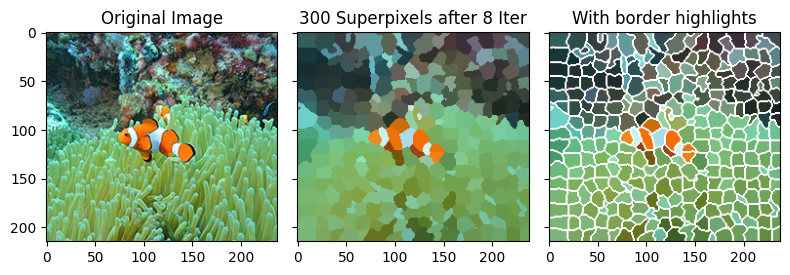

With 300 superpixels, the image is recognizable from the superpixel colors alone, and the borders follow the strong edges, like the outlines of the fish and the stripes on them, while staying fairly compact in flat regions.

Compare with `skimage`¶

skimage.segmentation.slic is a fast, polished implementation of the same algorithm, working in Lab color and enforcing connectivity. Its compactness parameter is the $m$ above.

from skimage.segmentation import slic, mark_boundaries

f, ax = plt.subplots(1, 3, figsize=(10, 3), sharex=True, sharey=True)
ax[0].imshow(IRwB / 255)
ax[0].set_title('Our SLIC')
for a, compactness in zip(ax[1:], [10, 30]):
    segments = slic(I / 255, n_segments=SUPERPIXELS, compactness=compactness, start_label=0)
    a.imshow(mark_boundaries(I / 255, segments))
    a.set_title(f'skimage, compactness={compactness}\n({segments.max() + 1} superpixels)', fontsize=9)
plt.tight_layout()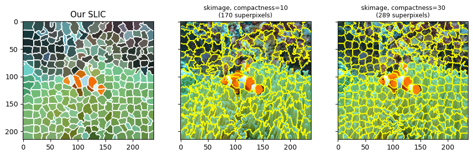

With compactness=30, skimage’s superpixels look much like ours: compact, nearly regular regions that bend to follow the strongest edges, like the outline of the fish. With compactness=10, color dominates. The superpixels wander to follow every color boundary in the busy anemone and coral, and they become very irregular. (skimage also merges tiny fragments, so you get somewhat fewer superpixels than requested.) Which is better depends on what you’ll use the superpixels for.

References¶

Achanta, R., Shaji, A., Smith, K., Lucchi, A., Fua, P., & Süsstrunk, S. (2012). SLIC Superpixels Compared to State-of-the-Art Superpixel Methods. IEEE Transactions on Pattern Analysis and Machine Intelligence, 34(11), 2274–2282. 10.1109/tpami.2012.120