Stough, 202-
The Lab colorspace is also oriented around adjusting color according to human vision perception as opposed to mechanism (r-g-b stimulus). It goes further than HSV or YCbCr, though. CIE L*a*b* (1976) was designed by the International Commission on Illumination (CIE) so that distances in the space match perceived differences in color. Two colors that look equally different to a typical human observer should be about equally far apart in Lab, wherever they are in the space. No RGB-derived space comes close to that.
Lab is built on two ideas from color science:
Opponent process: after the three kinds of cones, our visual system encodes color as three opponent signals: light vs. dark, red vs. green, and yellow vs. blue. (That’s why there’s no such thing as a “reddish green” or a “yellowish blue”.) Lab’s three axes are these: is lightness from 0 (black) to 100 (white), runs from green (negative) to red (positive), and from blue (negative) to yellow (positive).
Nonlinear response: our perception of lightness is roughly a cube root of physical intensity. We’re much more sensitive to changes among dark tones than among bright ones, and builds that in.
%matplotlib inline
import matplotlib.pyplot as plt
import numpy as np
import skimage.color as color
import matplotlib.colors as mcolors

# For importing from alternative directory sources
import sys
sys.path.insert(0, '../dip_utils')

from matrix_utils import arr_info
from vis_utils import (vis_lab_cube,
                       vis_hists,
                       lab_uniform)
The L*a*b* Channels
IMAGE = 'mountainSpring.jpg'
# IMAGE = 'peppers.png'

# Let's construct our own colormaps
cm_KR = mcolors.LinearSegmentedColormap.from_list('kr', [(0,0,0), (1, 0, 0)], 256)
cm_KG = mcolors.LinearSegmentedColormap.from_list('kg', [(0,0,0), (0, 1, 0)], 256)
cm_KB = mcolors.LinearSegmentedColormap.from_list('kb', [(0,0,0), (0, 0, 1)], 256)
Irgb = plt.imread('../dip_pics/' + IMAGE)
# Image of uniform random distributed color
# Irgb = np.random.random((100,100,3))# Let's construct our own colormaps for the a and b dimensions.
colorsA = [(0,1,0), (.5,.5,.5), (1,0,0)] # green -> red
colorsB = [(0,0,1), (.5,.5,.5), (1,1,0)] # blue -> yellow
cmA = mcolors.LinearSegmentedColormap.from_list('GreenRed', lab_uniform(colorsA), 256)
cmB = mcolors.LinearSegmentedColormap.from_list('BlueYellow', lab_uniform(colorsB), 256)f, ax = plt.subplots(3,3, figsize = (8,6), sharex=True, sharey=True, num='RGB vs L*a*b*')
Ilab = color.rgb2lab(Irgb)
# Row 0: just the full color image
ax[0][1].imshow(Irgb)
ax[0][0].set_axis_off()
ax[0][2].set_axis_off()
# Row 1: r g b channels
for i in range(3):
ax[1,i].imshow(Irgb[...,i], cmap=[cm_KR, cm_KG, cm_KB][i])
ax[1,i].set_title(['Red', 'Green', 'Blue'][i])
# Now to display the HSV space.
ax[2,0].imshow(Ilab[...,0], cmap='gray')
ax[2,0].set_title('L')
ax[2,1].imshow(Ilab[...,1], cmap=cmA)
ax[2,1].set_title('a - green->red')
ax[2,2].imshow(Ilab[...,2], cmap=cmB)
ax[2,2].set_title('b - blue->yellow')
plt.tight_layout()
# These attempts for figure title may no longer be supported.
# f.canvas.set_window_title('RGB vs L*a*b*')
# f.suptitle('RGB vs L*a*b*')
plt.show()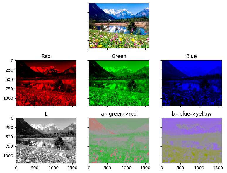
As with in YCbCr, the channel carries the detail and looks like a natural grayscale photo. The two color channels read like the opponent signals they’re named for: in the meadow is greenish (negative), the flowers stand out red-ish, and the sky and snow sit near neutral. In the sky is strongly blue (negative), while the sunlit grass and yellow flowers push toward yellow.
Let’s check the ranges:
for i, name in enumerate(['L*', 'a*', 'b*']):
    print(f'{name}: [{Ilab[...,i].min():7.2f}, {Ilab[...,i].max():7.2f}]')
L*: [ 0.00, 100.00]
a*: [ -64.93, 89.25]
b*: [ -71.62, 94.48]
is in , and and are signed, with 0 meaning neutral gray. Unlike RGB and YCbCr, Lab values aren’t bytes, so we keep them as floats. Converting from RGB goes through the CIE XYZ space and involves the cube-root nonlinearity, so Lab is not just a matrix multiply away from RGB.
Let’s visualize in 3D
vis_lab_cube(Irgb)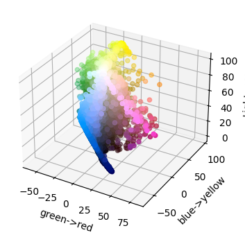
vis_lab_cube(np.random.random((100,100,3)))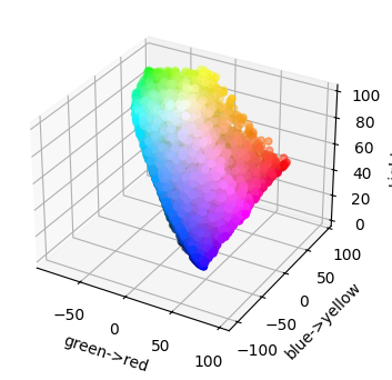
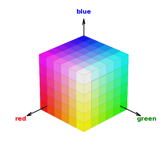
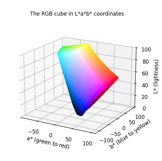
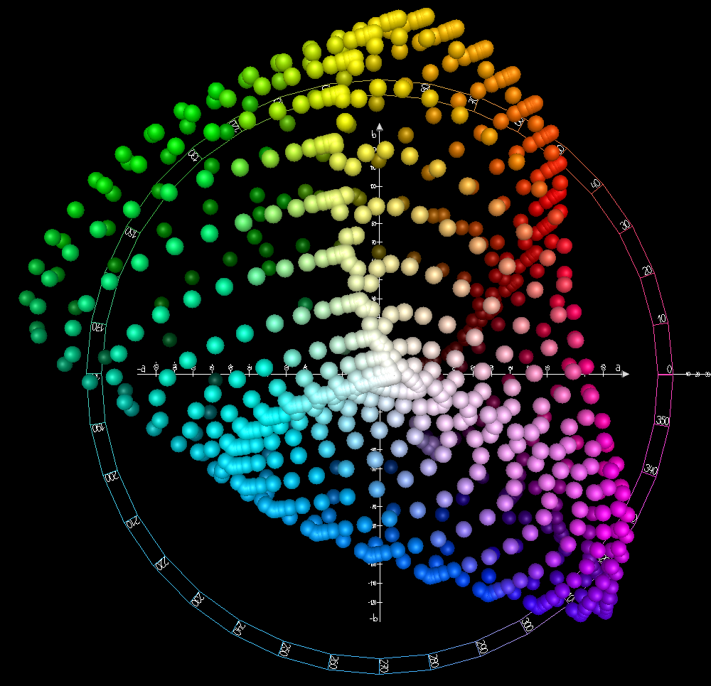
The 3D view shows why this space is strange-looking. The RGB cube, which is what our display can actually show, becomes a lopsided, twisted shape in Lab. It’s tall and narrow in some hues and bulging in others, because the cube’s equal steps are not perceptually equal steps.
Perceptual Uniformity and Color Difference
What does “perceptually uniform” buy us? Consider two pairs of colors, each pair differing by exactly the same amount (0.1) in a single RGB channel: two greens and two blues.
pairs = {'greens': ([0, .6, 0], [0, .7, 0]),
         'blues':  ([0, 0, .6], [0, 0, .7])}

f, ax = plt.subplots(1, 2, figsize=(6,2))
for a, (name, (c1, c2)) in zip(ax, pairs.items()):
    a.imshow(np.array([[c1, c2]]))
    lab1, lab2 = color.rgb2lab(np.array([[c1]])), color.rgb2lab(np.array([[c2]]))
    dE76 = color.deltaE_cie76(lab1, lab2).item()
    dE00 = color.deltaE_ciede2000(lab1, lab2).item()
    a.set_title(f'{name}\n$\\Delta E_{{76}}$={dE76:.1f}, $\\Delta E_{{00}}$={dE00:.1f}', fontsize=9)
    a.set_axis_off()
plt.tight_layout()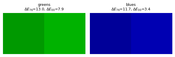
To most people the two greens look clearly different, while the two blues are much harder to tell apart, even though in RGB both pairs are exactly 0.1 apart. Lab captures that difference.
The simplest perceptual color difference, , is just the Euclidean distance in Lab:
A of about 1 to 2.3 is often quoted as a “just noticeable difference”. Lab turned out to be not perfectly uniform, especially in saturated blues, so the CIE later refined the distance formula itself, most recently as (CIEDE2000). The blue pair shows why: rates the two pairs as similarly different, but agrees with our eyes that the blues are much closer. Both are available in skimage.color as deltaE_cie76 and deltaE_ciede2000.
This is why Lab shows up wherever “how different do these colors look?” matters: color quality control in printing and manufacturing, choosing colormaps (our own lab_uniform helper in vis_utils uses it to equalize perceived brightness across a colormap, as in the YCbCr notebook), and clustering pixels by color, which we’ll do with SLIC superpixels.
Illuminants and the White Point
There’s a subtlety hiding in every conversion to Lab: what counts as white? A sheet of white paper reflects very different light under noon daylight, an overcast sky, or an incandescent bulb, yet our visual system adapts so that it still looks white. Lab handles this by defining every color relative to a reference white, given by a standard illuminant.
The CIE standardized several illuminants as spectra of light. The most common are:
D65: average noon daylight (about 6500K), the white point of sRGB and of most displays. This is
skimage’s default;D50: “horizon” daylight (about 5000K), slightly warmer, standard in the printing industry;
A: a tungsten incandescent bulb (about 2856K), very warm/orange.
Here are their white points in CIE XYZ, where (luminance) is normalized to 1:
for ill in ['D65', 'D50', 'A']:
    print(ill, color.xyz_tristimulus_values(illuminant=ill, observer='2').round(3))
D65 [0.95 1. 1.089]
D50 [0.964 1. 0.825]
A [1.098 1. 0.356]
Illuminant A has far less short-wavelength (bluish) light, hence its much smaller .
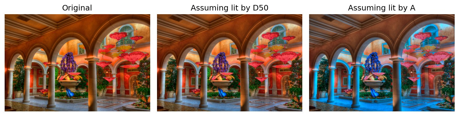
We can use this to white balance an image. rgb2lab(I, illuminant=X) interprets the image’s colors relative to white point , and lab2rgb(lab, illuminant='D65') renders those relative colors for a D65 display. The net effect is to scale the image’s XYZ values by the ratio of the two white points, a simple form of chromatic adaptation. This image of the Bellagio has a strong warm cast. Let’s see what happens if we assume it was lit by a warmer illuminant.
I = plt.imread('../dip_pics/bellagio.jpg') / 255.0

f, ax = plt.subplots(1, 3, figsize=(10,3), sharex=True, sharey=True)
ax[0].imshow(I)
ax[0].set_title('Original')
for a, ill in zip(ax[1:], ['D50', 'A']):
    J = color.lab2rgb(color.rgb2lab(I, illuminant=ill), illuminant='D65')
    a.imshow(np.clip(J, 0, 1))
    a.set_title(f'Assuming lit by {ill}')
[a.set_axis_off() for a in ax];
plt.tight_layout()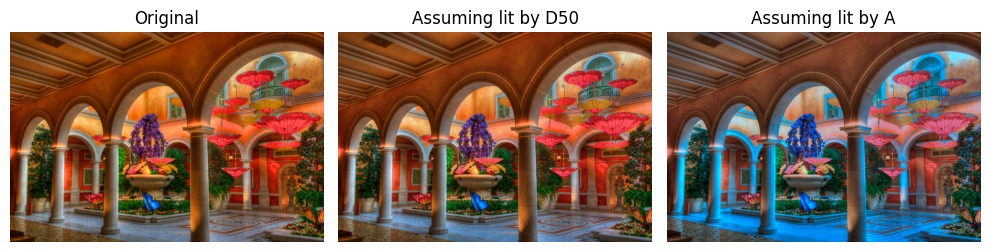
Assuming a D50 light source cools the image slightly, taking the edge off the orange. Assuming illuminant A overcorrects dramatically: the scene wasn’t really lit by bare tungsten bulbs, so compensating for one pushes all the bright areas toward cyan. Your camera’s “white balance” setting is making this same kind of guess about the illuminant every time you take a picture.