Playing with Color

stough 202-

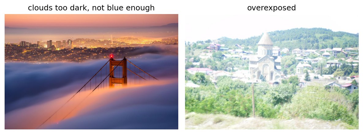
In this activity we’ll use what we’ve learned about color to try and enhance an image or even compress it without too much perceptual loss. The other notebooks in this folder should be useful here, particularly color_intro, color_HSV, and color_YCbCr.

Imports¶

You can borrow the imports from any of the other notebooks in this directory.

1. Enhancement: Improving the Color of an Image¶

Take a look at ../dip_pics/sf.jpg and try the vis_hists function on it to the distributions of the R,G,B channels. Of course you can try this out with any image you like of course.

To me it looks like the clouds shrouding the Golden Gate Bridge are too dark, not blue enough really for my tastes. You can see this in the relative color distributions as well, with the blue component maxing out below the midpoint of the intensity range.

Try adding some blue to the image to really make those clouds pop better. Be careful to use the arr_info to understand both the dtype and understood range of your data. (In fact, now might be a good time to review the matplotlib_tutorial on the kind of data imshow and our vis_image.)

2. Ehancement: Improving Contrast through Saturation of Color¶

Take a look at ../dip_pics/world_overexposed.jpg. Here we have a very overexposed image. (Again, find any overexposed image you like). What this means generally is that we have a lot of what should be color/Hue showing up as mostly white; as in, it’s been mixed with too much white. See the color_HSV demo titled “Viewing the planes of the HSV space” and see what happens as saturation $S_{HSV}$ approaches zero.

Try converting the image to HSV and then scaling the saturation component to improve the color purity of all those washed-out pixels. Then convert back to RGB and see if it’s improved. Remember, from the skimage documentation, that the hsv channels are all in $[0,1]$, so when you do the scaling you might need to [np.clip]https://numpy.org/doc/stable/reference/generated/numpy.clip.html).

3. Compression: Reducing the Bit-Depth of an Image to Save Space¶

In a prior activity we reduced the bit-depth of the RGB color channels of an image and saw how that quantization affected the image quality, creating sharp edges of color change in what would be smoothly graded areas. So one of the limits of potentially compressing images relates to the minimum bit-depth that can maintain perceptual fidelity.

But in this module’s materials, we’ve seen that some color spaces (HSV, YCbCr, and Lab*) include some dimension that captures the brightness/luminance/intensity representation of an image separately from the “color” aspect. YCbCr in particular is used a lot in compression for precisely this reason.

In the below cells, try considering an image like ../dip_pics/bellagio.jpg or ../dip_pics/mountainSpring.jpg for example.

• See what happens when you reduce the bit-depth to 4-4-4 in RGB.

• Then try reducing the bit-depth to 6-3-3 but in the YCbCr space. Here we’re saving the same number of bits per pixel, but differentially quantizing (and therefore compressing) the Luminance and color components.

It may be useful here to define a function that quantizes a 2D ndarray instead of a whole image at once. Luckily, it’s likely the same quantization function you’ve already written may suffice. I include a useable version here just to help.

Be careful: skimage.color.ycbcr2rgb expects ‘float64’ data type.