YCbCr - Y: Luminance; Cb: Chrominance-Blue; and Cr: Chrominance-Red Colorspace

Stough, 202-

The YCbCr colorspace is also oriented around adjusting color according to human vision perception as opposed to mechanism (r-g-b stimulus). Where HSV is built for describing and choosing colors, YCbCr is built for transmitting and compressing them. It’s the colorspace inside JPEG images and nearly all digital video.

The idea is to separate an image into one channel of brightness, the luma $Y$ , and two channels of color difference, the chroma $C_b$ (how much bluer than gray) and $C_r$ (how much redder than gray). Our visual system is far more sensitive to fine detail in brightness than in color, so once they’re separated we can afford to store the chroma channels with much less detail. We’ll see that directly at the end of this notebook.

%matplotlib inline
import numpy as np
import matplotlib.pyplot as plt
import skimage.color as color
import matplotlib.colors as mcolors

# For importing from alternative directory sources
import sys  
sys.path.insert(0, '../dip_utils')

from matrix_utils import arr_info
from vis_utils import (vis_rgb_cube,
                       vis_ybr_cube,
                       vis_hists,
                       lab_uniform)

IMAGE = 'mountainSpring.jpg'
# IMAGE = 'peppers.png'

# Let's construct our own colormaps
cm_KR = mcolors.LinearSegmentedColormap.from_list('kr', [(0,0,0), (1, 0, 0)], 256)
cm_KG = mcolors.LinearSegmentedColormap.from_list('kg', [(0,0,0), (0, 1, 0)], 256)
cm_KB = mcolors.LinearSegmentedColormap.from_list('kb', [(0,0,0), (0, 0, 1)], 256)

Irgb = plt.imread('../dip_pics/' + IMAGE)

# Image of uniform random distributed color
# Irgb = np.random.random((100,100,3))

The Conversion¶

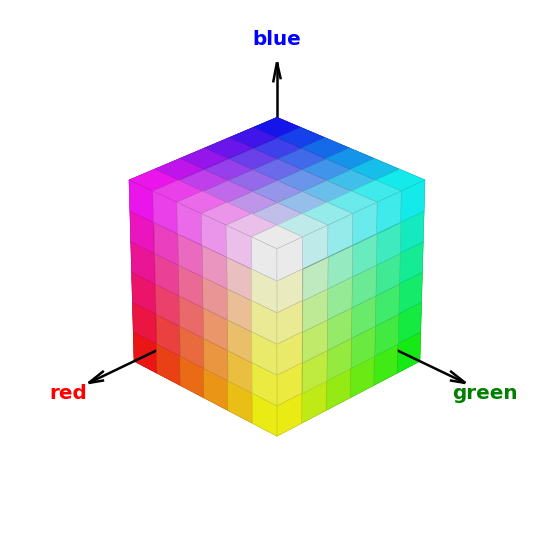
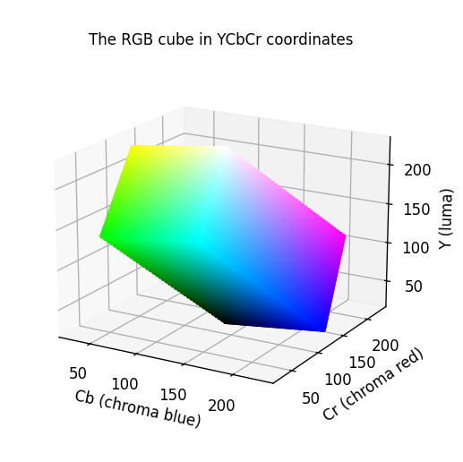
YCbCr is just a linear transform of RGB, plus an offset: a rotation, scaling, and shift of the RGB cube. skimage uses the ITU-R BT.601 standard, which for $R,G,B \in [0,1]$ gives

\begin{bmatrix} Y \\ C_b \\ C_r \end{bmatrix} = \begin{bmatrix} 16 \\ 128 \\ 128 \end{bmatrix} + \begin{bmatrix} 65.481 & 128.553 & 24.966 \\ -37.797 & -74.203 & 112.0 \\ 112.0 & -93.786 & -18.214 \end{bmatrix} \begin{bmatrix} R \\ G \\ B \end{bmatrix}

A few things to notice:

The $Y$ row is a weighted sum with green weighted most and blue least, matching the eye’s sensitivity to each. A pure green pixel is perceived as much brighter than a pure blue one of the same intensity.
The $C_b$ and $C_r$ rows each sum to zero. Any gray pixel ( $R=G=B$ ) therefore has $C_b = C_r = 128$ : no color, only brightness.
The ranges are $Y \in [16, 235]$ and $C_b, C_r \in [16, 240]$ , a convention inherited from analog video that leaves some headroom at either end. (JPEG uses a slightly different “full-range” variant over $[0,255]$ .)

Let’s check this with pure red, green, blue, white and black.

rgb = np.array([[[1,0,0], [0,1,0], [0,0,1], [1,1,1], [0,0,0]]], dtype=float)
color.rgb2ycbcr(rgb).round(1)

array([[[ 81.5,  90.2, 240. ],
        [144.6,  53.8,  34.2],
        [ 41. , 240. , 109.8],
        [235. , 128. , 128. ],
        [ 16. , 128. , 128. ]]])

White and black land at $Y=235$ and $Y=16$ with neutral chroma $(128,128)$ , as promised, and green has by far the largest luma of the three primaries.

Cb and Cr colormaps¶

I’m going to be careful here with the colormap to have a perceptually constant transition between yellow and blue (Cb) and cyan and red (Cr). I don’t want one side to be perceptually brighter than the other.

# Let's construct our own colormaps for the a and b dimensions.
# I'm going to be careful with my color,  
colorsCb = [(.7, .7, 0), (.6,.6,1)]
colorsCr = [(0, .7, .7), (1,.4,.4)]

cmCb = mcolors.LinearSegmentedColormap.from_list('Cb', lab_uniform(colorsCb), 256)
cmCr = mcolors.LinearSegmentedColormap.from_list('Cr', lab_uniform(colorsCr), 256)

f, ax = plt.subplots(3,3, figsize = (8,6), sharex=True, sharey=True, num = 'RGB vs YCbCr')

Iybr = color.rgb2ycbcr(Irgb)

# Row 0: just the full color image
ax[0][1].imshow(Irgb)
ax[0][0].set_axis_off()
ax[0][2].set_axis_off()

# Row 1: r g b channels
for i in range(3):
    ax[1,i].imshow(Irgb[...,i], cmap=[cm_KR, cm_KG, cm_KB][i])
    ax[1,i].set_title(['Red', 'Green', 'Blue'][i])


# Now to display the HSV space.

ax[2,0].imshow(Iybr[...,0], cmap='gray')
ax[2,0].set_title('Y')

ax[2,1].imshow(Iybr[...,1], cmap=cmCb)
ax[2,1].set_title('Cb - yellow->blue')

ax[2,2].imshow(Iybr[...,2], cmap=cmCr)
ax[2,2].set_title('Cr - cyan->red')

plt.tight_layout()
# f.canvas.set_window_title('RGB vs YCbCr')
plt.show()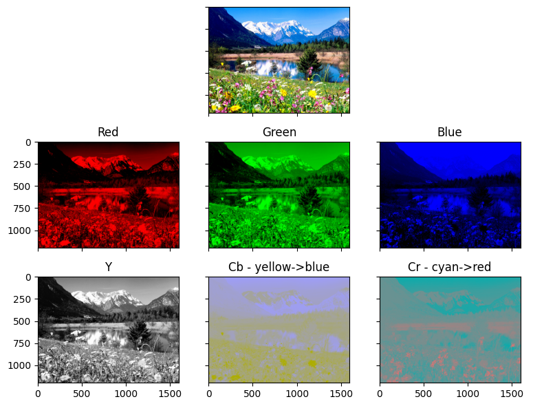

The $Y$ channel looks like a natural grayscale version of the image, with nearly all the detail: every flower petal, every ridge of the mountains. The chroma channels, by contrast, look smooth and blotchy. They mostly say “this region is bluish, this region is greenish”. That observation is the whole reason YCbCr exists.

Let’s visualize in 3D¶

vis_ybr_cube(Irgb)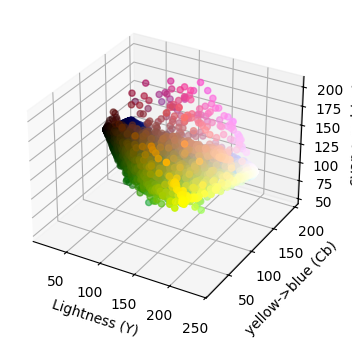

vis_ybr_cube(np.random.random((100,100,3)))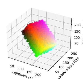

View the Cb-Cr plane for various Y¶

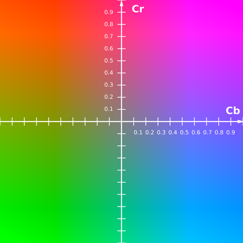
The visualization of the YCbCr space is a bit weird, because it looks just like the rgb color cube, but maybe rotated, translated, and stretched a little. So I’m trying here to visualize the CbCr plane for any luma Y. skimage notes that Y must be in 16-235. Also, when you transform back you could get out-of-range values for r,g,b. Normally these get clipped to show a CbCr plane like below, but a lot of that plane is invalid. So here, I’ll show the whole (clipped to 0-1) plane and then also just the valid part (within the color cube). What we’re doing here is taking slices orthogonal to the Luminance direction.

def clipRGB(rgb):
    toosmall = np.any(rgb<0, axis=2)
    toobig = np.any(rgb>1, axis=2)
    rgb[toobig | toosmall, :] = 0
    return rgb

from ipywidgets import VBox, IntSlider

pass  # (static) plt.ioff()
# plt.clf()

y_slider = IntSlider(
    orientation='horizontal',
    value=150,
    min=16,
    max=235,
    step=1,
    description='Y (Lightness)'
)


# Initialize globals
Cb, Cr = np.meshgrid(range(256), range(256), indexing='xy')
ybr = np.stack([150*np.ones((256,256)), Cb[::-1,:], Cr[::-1,:]], axis=2)
rgb = color.ycbcr2rgb(ybr)

# Make figure.
fig_args = {'num':' ', 'frameon':True, 'sharex':True, 'sharey':True}
fig, ax = plt.subplots(1,2, figsize=(8,4), **fig_args) 
plt.tight_layout()


# display artists
ldisp = ax[0].imshow(np.clip(rgb,0,1))
ax[0].set_title('CbCr plane')
rdisp = ax[1].imshow(clipRGB(rgb))
rtext = ax[1].set_title(f'Valid at Y {150:03d}')

# Update function.
def update_image(change):
    global ybr, rgb, ldisp, rdisp, rtext
    
    ybr = np.stack([change.new*np.ones((256,256)), Cb[::-1,:], Cr[::-1,:]], axis=2)
    rgb = color.ycbcr2rgb(ybr)
    
    ldisp.set_array(np.clip(rgb,0,1))
    rdisp.set_array(clipRGB(rgb))
    rtext.set_text(f'Valid at Y {change.new:03d}')
    fig.canvas.draw()
    fig.canvas.flush_events()

y_slider.observe(update_image, names='value')

pass  # (static) VBox([y_slider, fig.canvas])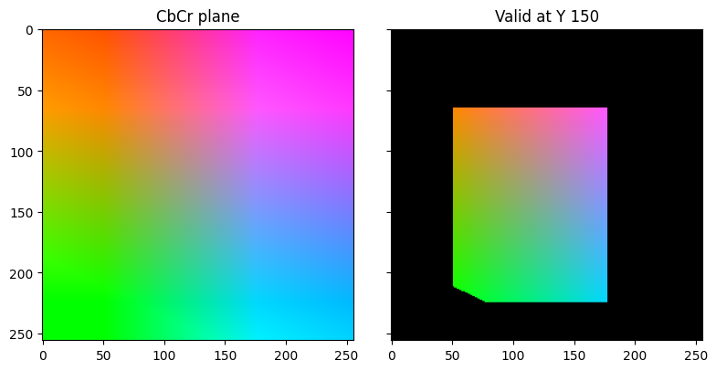

# Turn interactive mode back on (the demo above turned it off), so new figures display.
plt.ion()

<contextlib.ExitStack at 0x7f4bdb5e5d60>

Chroma Subsampling¶

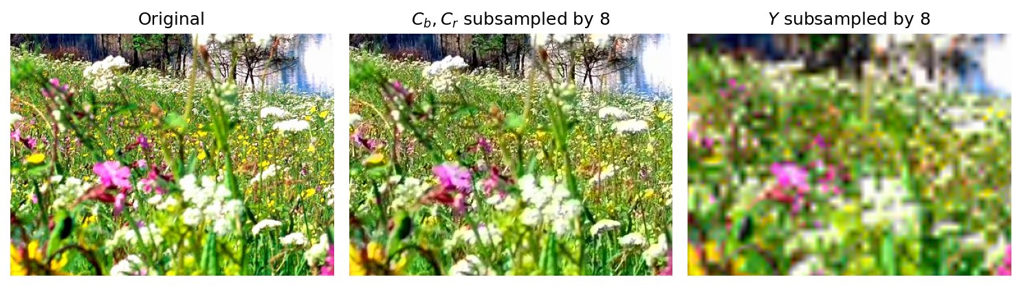
Here’s the payoff. Let’s throw away most of the color information: keep only every 8th row and column of $C_b$ and $C_r$ (that’s $\frac{1}{64}$ of the chroma samples), then scale them back up to full size and convert back to RGB. For comparison, we’ll do the same thing to $Y$ instead, leaving the chroma alone.

from skimage.transform import resize

def subsample(C, k=8):
    # Keep every kth sample, then (bilinearly) scale back up to the original size.
    return resize(C[::k, ::k], C.shape, order=1)

I = Irgb / 255.0
ybr = color.rgb2ycbcr(I)

ybr_chroma = ybr.copy()
ybr_chroma[..., 1] = subsample(ybr[..., 1])
ybr_chroma[..., 2] = subsample(ybr[..., 2])

ybr_luma = ybr.copy()
ybr_luma[..., 0] = subsample(ybr[..., 0])

I_chroma = np.clip(color.ycbcr2rgb(ybr_chroma), 0, 1)
I_luma = np.clip(color.ycbcr2rgb(ybr_luma), 0, 1)

crop = (slice(700, 1000), slice(200, 600))  # zoom in on the flowers
f, ax = plt.subplots(1, 3, figsize=(10,3), sharex=True, sharey=True)
for a, J, title in zip(ax, [I, I_chroma, I_luma], ['Original', '$C_b, C_r$ subsampled by 8', '$Y$ subsampled by 8']):
    a.imshow(J[crop])
    a.set_title(title)
    a.set_axis_off()
plt.tight_layout()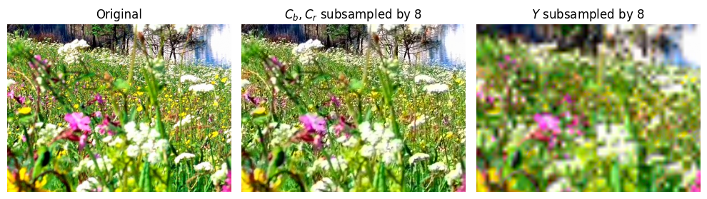

Discarding $\frac{63}{64}$ of the color samples is nearly invisible. You may spot a little color bleeding at the edges of the brightest petals if you look closely. Doing the same thing to brightness wrecks the image. Measured as mean squared error, the luma-subsampled image is roughly eight times worse.

This is exactly what JPEG and video codecs do. The common “4:2:0” scheme keeps $Y$ at full resolution but stores $C_b$ and $C_r$ at half resolution in each direction, cutting the total data in half before any other compression even begins.