HSV - Hue, Saturation, Value Colorspace

Stough, 202-

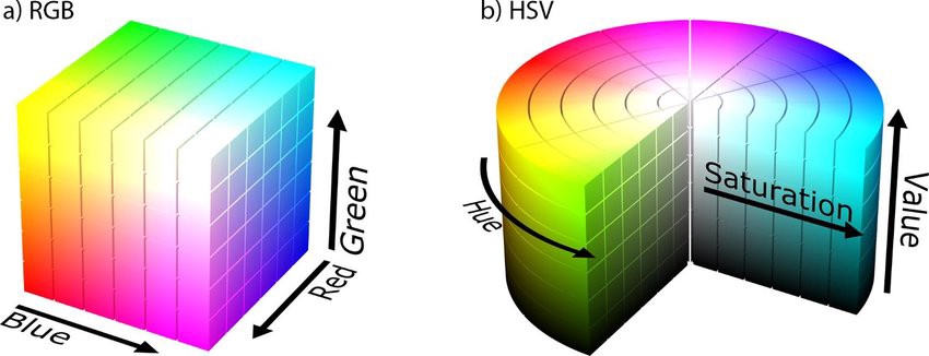
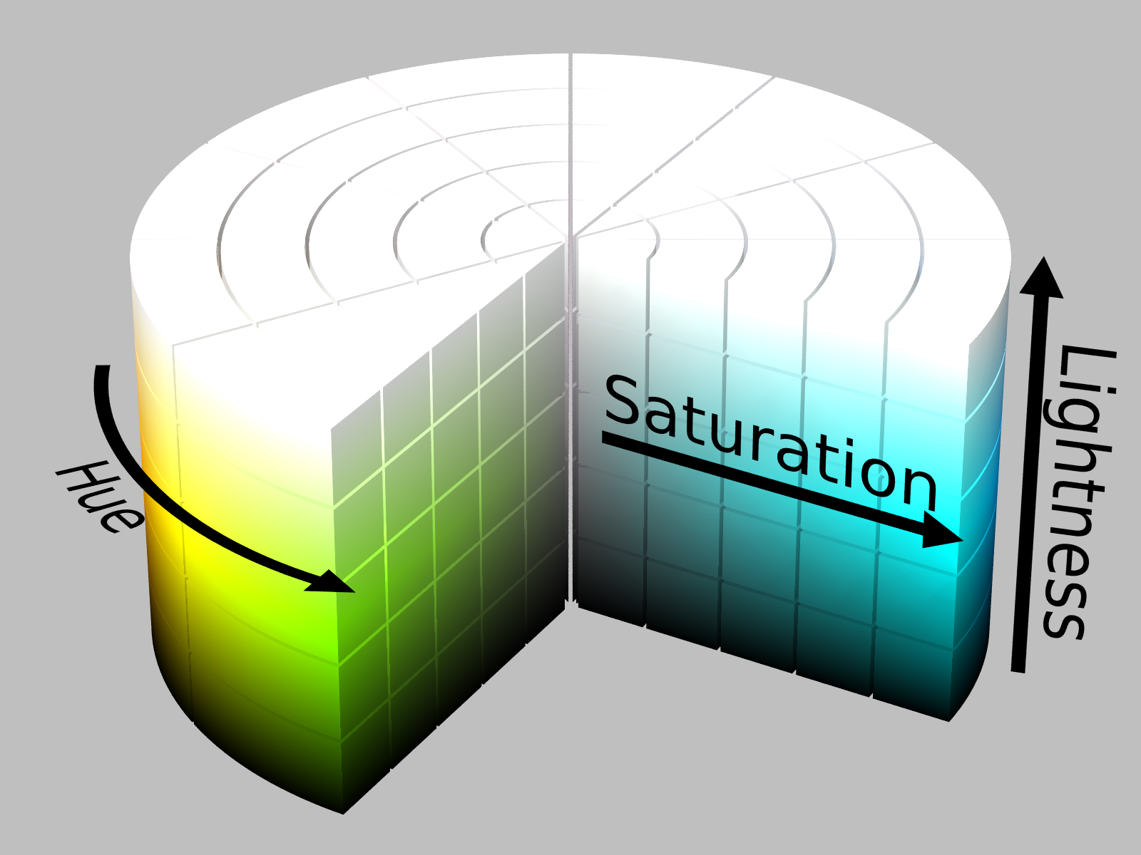
The HSV and closely related HSL colorspaces are ways of considering ‘color’ that separate the brightness of a color from its tone and purity. This is useful because we as humans are highly attuned to brightness changes in our perception. So if the RGB space speaks to the mechanism by which we receive a color stimulus--activation of red, green, and blue-centered cones--then the HSV speaks more to how we perceive or speak about color.

%matplotlib inline
import matplotlib.pyplot as plt
import numpy as np
import matplotlib.colors as mcolors
import skimage.color as color
from ipywidgets import VBox, HBox, FloatSlider

# Enable LaTeX rendering in matplotlib
# Seems to be unneeded, and doesn't fix the issue with
# the FloatSlider widget description text displaying incorrectly. 
# import matplotlib as mpl
# mpl.rcParams['text.usetex'] = True

# For importing from alternative directory sources
import sys  
sys.path.insert(0, '../dip_utils')

from matrix_utils import arr_info
from vis_utils import (vis_rgb_cube,
                       vis_hsv_cube,
                       vis_hists,
                       lab_uniform)

Viewing the planes of the HSV space.¶

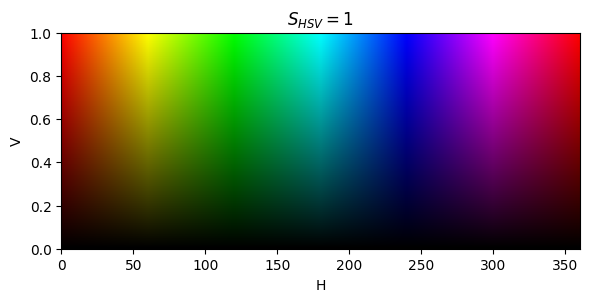
Here I’ll make a little interactive plot on the HSV space for various saturation, thanks to HYRY’s stackoverflow answer. We first stack together an HSV image, then convert to RGB so that we can display it.

There is a bit of a problem with these demos. The plt.ioff() and plt.ion() are required to avoid duplication of plots when putting together an interactive demo. plt.close() is used to make sure those plots don’t regenerate later in the notebook.

def changeSat(HSV, newvalue=1.0):
    H, S, V = np.split(HSV, indices_or_sections=3, axis=-1)
    S = newvalue*np.ones_like(V)
    HSV = np.dstack((H,S,V))
    return color.hsv2rgb(HSV)

pass  # (static) plt.ioff()
# plt.clf()

# Set up the initial display
V, H = np.mgrid[0:1:100j, 0:1:360j]
S = np.ones_like(V)
HSV = np.dstack((H,S,V))
RGB = color.hsv2rgb(HSV)


# A slider to set the saturation.
sat_slider = FloatSlider(
    orientation='horizontal',
    value=1.0,
    min=0.00,
    max=1.00,
    step=0.01,
    description='S_HSV'
)

# Setting up the figure.
fig_args = {'num':1, 'frameon':True}
fig, ax = plt.subplots(1,1, figsize=(6,3), **fig_args)
fig.canvas.header_visible = False

thedisp = ax.imshow(RGB, origin='lower', extent=[0, 360, 0, 1], aspect=150)
plt.xlabel('H') # These don't need to change
plt.ylabel('V')
thetext = ax.set_title('$S_{HSV}=1$')
plt.tight_layout()

def update_image(change):
    global thedisp, thetext, HSV
    
    I_rgb = changeSat(HSV, change.new)
    thedisp.set_array(I_rgb)
    thetext.set_text(f'$S_{{HSV}}$={change.new:.02f}')
    fig.canvas.draw()
    fig.canvas.flush_events()

sat_slider.observe(update_image, names='value')

pass  # (static) VBox([sat_slider, fig.canvas])

# Close the above interactive demo figure, so that it won't appear later.
plt.close(1)

Drag the saturation slider down and watch what happens: every hue fades toward gray, and at $S_{HSV}=0$ the whole plot is just a vertical grayscale ramp, the same at every hue. With no saturation, hue has no effect at all. Remember this; it comes back to bite us below.

Note also that red appears at both the left ( $H=0$ ) and right ( $H=360$ ) edges. Hue is an angle, so $0°$ and $360°$ are the same color. That’s why the HSL/HSV diagrams above draw hue around a circle.

Viewing an image as RGB and HSV for comparison¶

IMAGE = 'mountainSpring.jpg'
# IMAGE = 'peppers.png'
# IMAGE = 'blueridge.jpg'

# Let's construct our own colormaps
cm_KR = mcolors.LinearSegmentedColormap.from_list('kr', [(0,0,0), (1, 0, 0)], 256)
cm_KG = mcolors.LinearSegmentedColormap.from_list('kg', [(0,0,0), (0, 1, 0)], 256)
cm_KB = mcolors.LinearSegmentedColormap.from_list('kb', [(0,0,0), (0, 0, 1)], 256)

Irgb = plt.imread('../dip_pics/' + IMAGE)

# Image of uniform random distributed color
# Irgb = np.random.random((100,100,3))

# plt.clf()
plt.ion()

f, ax = plt.subplots(3,3, figsize = (8,6), sharex=True, sharey=True, num='RGB vs HSV')

Ihsv = color.rgb2hsv(Irgb)

# Row 0: just the full color image
ax[0][1].imshow(Irgb)
ax[0][0].set_axis_off()
ax[0][2].set_axis_off()

# Row 1: r g b channels
for i in range(3):
    ax[1,i].imshow(Irgb[...,i], cmap=[cm_KR, cm_KG, cm_KB][i])
    ax[1,i].set_title(['Red', 'Green', 'Blue'][i])


# Now to display the HSV space.

cmapNameHue = 'myHue'
colorsH = [(.7,0,0), (.5,.5,0), (0,.7,0), (0,.5,.5), (0,0,.7), (.5, 0, .5), (.7, 0, 0)]
cmHue = mcolors.LinearSegmentedColormap.from_list(cmapNameHue, lab_uniform(colorsH), 256)


ax[2,0].imshow(Ihsv[...,0], cmap=cmHue)
ax[2,0].set_title('H')

ax[2,1].imshow(Ihsv[...,1], cmap='gray')
ax[2,1].set_title('S')

ax[2,2].imshow(Ihsv[...,2], cmap='gray')
ax[2,2].set_title('V')

plt.tight_layout()
# These attempts for figure title may no longer be supported.
# f.canvas.set_window_title('RGB vs HSV')
# f.suptitle('RGB vs HSV')
plt.show()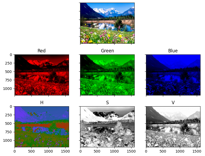

arr_info(Ihsv)

((1200, 1600, 3), dtype('float64'), np.float64(0.0), np.float64(1.0))

How the conversion works¶

rgb2hsv (like most libraries) works with RGB scaled to $[0,1]$ and returns $H$ , $S$ , $V$ also each in $[0,1]$ , so $H=1$ means $360°$ . For a pixel, let $M = \max(R,G,B)$ and $m = \min(R,G,B)$ . Then

V = M, \qquad S = \begin{cases} \frac{M - m}{M} & M > 0 \\ 0 & M = 0 \end{cases}

and the hue is an angle determined by which channel is largest, and by how the other two compare:

H = \frac{1}{6} \times \begin{cases} \frac{G - B}{M - m} \pmod 6 & M = R \\ \frac{B - R}{M - m} + 2 & M = G \\ \frac{R - G}{M - m} + 4 & M = B \end{cases}

So value is simply the brightest channel, saturation is how far apart the channels are relative to that, and hue says which part of the color wheel (red at 0, green at $\frac{1}{3}$ , blue at $\frac{2}{3}$ ) the pixel leans toward. We can confirm the first of these directly:

np.allclose(Ihsv[...,2], Irgb.max(axis=-1)/255)

True

Now look back at the figure. A few things to notice:

V looks like a grayscale version of the image, but not quite the one you’d expect. The snow, clouds, and the saturated flowers are all bright, since each has at least one channel near the max.
S is dark where the image is colorless (snow, clouds, the bright reflections), and bright for the deep blue sky, the green meadow, and the flowers.
H cleanly separates blue sky, green grass and pink/yellow flowers. But look at the snow and clouds: the hue there is a noisy speckle. When $M - m$ is tiny, which is exactly when $S$ is near 0, the hue formula divides small, noisy differences by a small number. For a gray pixel hue is simply undefined (skimage reports 0). Hue is only meaningful where there’s enough saturation to have a color in the first place.

That last point matters whenever you use hue to find things in an image, e.g. “find all the green pixels”. You almost always want to also require a minimum saturation (and value).

Let’s visualize in 3D¶

Given the HSV graph above, The Hue and Saturation can be seen in polar coordinates, with Hue as the angle $\theta$ and Saturation as the radius $R$ in. The Value coordinate (brightness) is the Z. Easy. So then, how to plot in polar coords? We’ve provided a nice library method vis_hsv_cube for just this. Read the link and understand the code.

vis_hsv_cube(Irgb)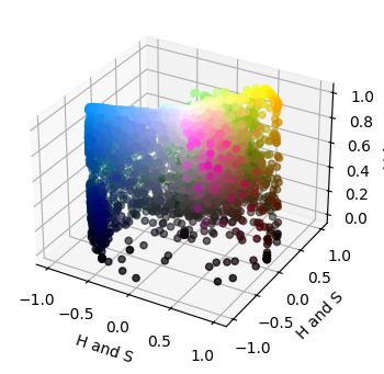

Problem: Manipulating the HSV components of an image...¶

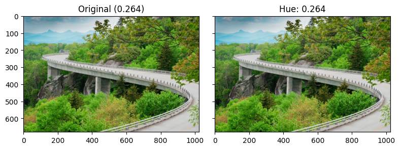
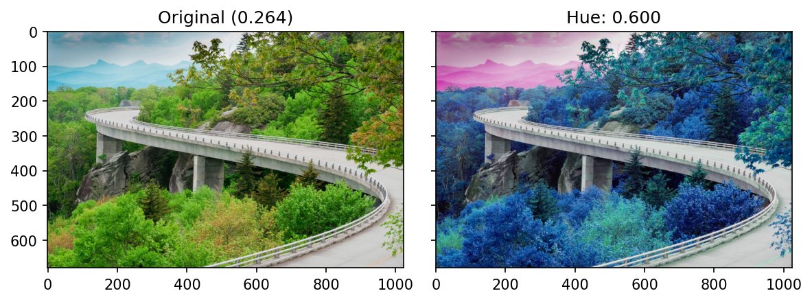
In the below interactive visualization we can manipulate the hue of an image. Try to complete the application by adding saturation and value sliders to this image manipulation tool.

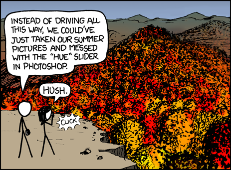
Thanks XKCD:

# I like this image more 
Irgb = plt.imread('../dip_pics/blueridge.jpg')
Ihsv = color.rgb2hsv(Irgb)

def changeHue(newhue):
    global Ihsv
    change = newhue - Ihsv[...,0].mean()
    
    Ic = Ihsv.copy()
    Ic[...,0] = np.fmod(Ic[...,0]+change, 1) # anything > 1 wraps around 0.
    
    return np.clip(Ic, 0, 1)

changeHue shifts every pixel’s hue by the same amount, the difference between the requested hue and the image’s mean hue. Because hue is an angle, we can’t just add and clip: a hue of 0.9 shifted by 0.2 should wrap around to 0.1, not saturate at 1.0. np.fmod(..., 1) does that wrap-around. Saturation and value are untouched, so the shadows, highlights, and textures of the scene all stay put while the colors rotate around the wheel.

pass  # (static) plt.ioff()
# plt.clf()

hue_mean = Ihsv[...,0].mean()

hue_slider = FloatSlider(
    orientation='horizontal',
    value=hue_mean,
    min=0.00,
    max=1.00,
    step=0.01,
    description='Hue'
)

fig_args = {'num':' ', 'frameon':True, 'sharex':True, 'sharey':True}
fig, ax = plt.subplots(1,2, figsize=(8,3), **fig_args) 

I_h = changeHue(hue_mean)
I_rgb = color.hsv2rgb(I_h)

# display artists I'll update
adisp = ax[0].imshow(Irgb)
rdisp = ax[1].imshow(I_rgb)

ax[0].set_title(f'Original ({hue_mean:.03f})')
rtext = ax[1].set_title(f'Hue: {hue_mean:.03f}')


def update_image(change):
    global Ihsv, I_h, adisp, rdisp, rtext
    
    I_rgb = color.hsv2rgb(changeHue(change.new)) 
    rdisp.set_array(I_rgb)
    rtext.set_text(f'Hue: {change.new:.03f}') #hue_slider.value
    fig.canvas.draw()
    fig.canvas.flush_events()

hue_slider.observe(update_image, names='value')

plt.tight_layout()

pass  # (static) VBox([hue_slider, fig.canvas])