Generic (e.g., non-linear) filtering - imageprocessing-awesome

stough 202-

Preview: Generic (e.g., non-linear) filtering

Defining and applying a generic filter
A non-linear filter: local standard deviation
🔨 Your Turn: Other Neighborhood Functions
🔨 Your Turn: Salt-and-Pepper Noise

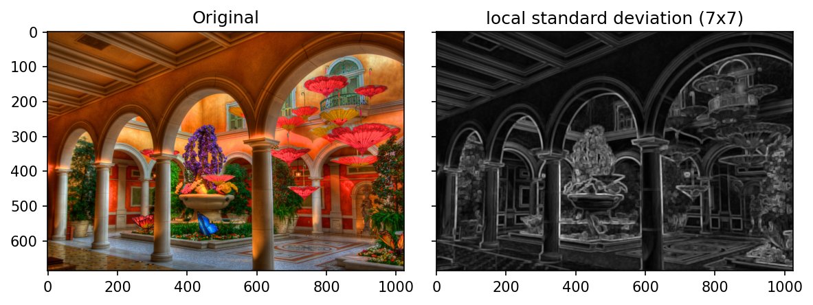
In this brief demo we use scipy.ndimage.generic_filter to compute non-linear filters on an image, such as min/max/median and others. This works a lot more slowly than the correlate we used for the linear filters.

Every filter we’ve used so far has been linear: each output pixel is a fixed weighted sum of its neighborhood, which is why a single kernel of weights describes the whole operation. But there are useful neighborhood operations that can’t be written as a weighted sum: the minimum or maximum of the neighborhood, its median, its range, and so on. These are non-linear filters. They still slide a window over the image and compute one output per pixel, but the computation can be any function of the pixels in the window.

%matplotlib inline
import matplotlib.pyplot as plt
import numpy as np

# For computing a generic filter on an image
from scipy.ndimage import generic_filter

# For importing from alternative directory sources
import sys  
sys.path.insert(0, '../dip_utils')

from matrix_utils import (arr_info,
                          make_linmap)
from vis_utils import (vis_rgb_cube,
                       vis_hists,
                       vis_pair)

Define the generic filtering function we want¶

This function will be applied to every footprint or neighborhood in the image. generic_filter hands the function a flat 1D array of the neighborhood’s values (121 of them for an $11 \times 11$ window), and the function returns a single number: the output pixel.

#simple blur
def mean_func(x):
    return x.mean()
#     xr = np.reshape(x, (5,5))
#     return np.mean(xr[:,3:])- np.mean(xr[:,:3])

def min_func(x):
    return x.min()

def max_func(x):
    return x.max()

def med_func(x):
    return np.median(x)

Apply the function to each channel separately.¶

We could alternatively define the footprint or size to the generic_filter call to include the separate channels (e.g., size = (3,3,3)), but it’s easier to think about this way.

We’ll also normalize the image to float $[0,1]$ for visualization purposes.

I = plt.imread('../dip_pics/bellagio.jpg').astype('float')
I = I/I.max()
arr_info(I)

((687, 1024, 3), dtype('float64'), np.float64(0.0), np.float64(1.0))

vis_hists(I)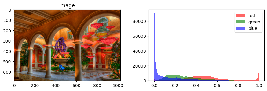

If = np.zeros(I.shape)
Out = np.zeros(I.shape[:2])

for chan in range(3):
    generic_filter(I[:, :, chan], function=mean_func, size=11, output=Out, mode='reflect')
    If[...,chan] = Out.copy();

vis_pair(I, If, second_title="mean filtered")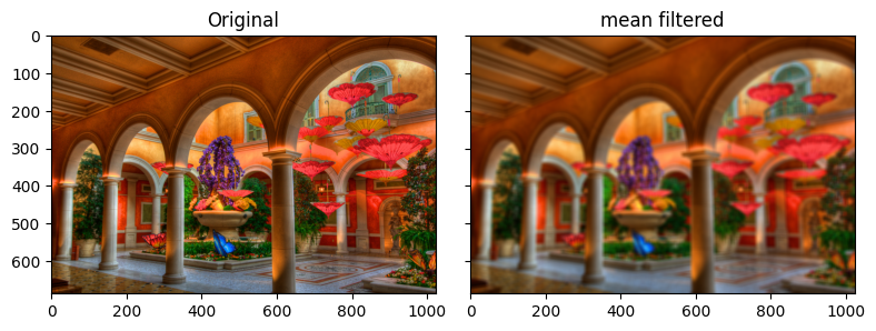

The mean filter gives the same result as correlating with the $11 \times 11$ box kernel in the low-pass demo, but it takes much longer to compute. correlate runs its loop over pixels in compiled C code, while generic_filter has to call our Python function once for every pixel of every channel. That’s millions of Python function calls for this image. (If you need a fast version of a common non-linear filter, scipy.ndimage has dedicated ones, such as median_filter, minimum_filter and maximum_filter.)

A Non-linear Filter: Local Standard Deviation¶

The mean is in fact a linear operator, so we’re not really looking into what these local non-linear operators can do for us yet. Let’s try one that isn’t: the standard deviation of the neighborhood,

\sigma_{i,j} = \sqrt{\frac{1}{n}\sum_{(k,l) \in N(i,j)} \left(p_{k,l} - \bar{p}_{i,j}\right)^2}

where $N(i,j)$ is the $n$ -pixel window around pixel $(i,j)$ and $\bar{p}_{i,j}$ is its mean. This measures how busy each neighborhood is: it is 0 wherever the window is flat, whatever the brightness, and large wherever the window straddles an edge or texture. No kernel of weights can compute it, because of the squaring and the square root. One way to see this: for any linear filter, filtering the sum of two images gives the sum of their filtered results, but the busyness of $I + J$ is not the busyness of $I$ plus the busyness of $J$ (think of $J = -I$ ).

We’ll compute it on a grayscale version of the image, with a $7 \times 7$ window, and time it.

import time

def std_func(x):
    return x.std()

Ig = I.mean(axis=2)  # a simple grayscale version

start = time.perf_counter()
S = generic_filter(Ig, function=std_func, size=7, mode='reflect')
print(f'generic_filter: {time.perf_counter() - start:.2f} seconds')
arr_info(S)

generic_filter: 16.04 seconds

((687, 1024),
 dtype('float64'),
 np.float64(0.002168262054284781),
 np.float64(0.29885254555571894))

vis_pair(I, S, cmap='gray', second_title='local standard deviation (7x7)')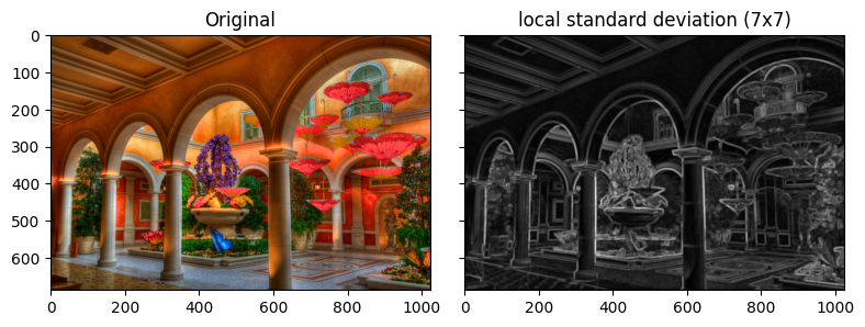

The local standard deviation is dark on the smooth walls and on the faces of the columns, and bright along the outlines of the arches and columns, the ceiling panels, and the umbrellas, flowers, and foliage. (Most of its values are small: half of the pixels are under 0.04, and the brightest edges reach about 0.3, on an image in $[0,1]$ .) A map like this is useful whenever we want to treat busy and flat regions differently: deciding where a compression scheme should spend its bits (compare the block transforms to come), where noise will be visible, or where one texture ends and another begins.

Building it from linear filters¶

Even though the standard deviation isn’t linear, we can assemble it from linear pieces. The variance is the mean of the squares minus the square of the mean,

\sigma^2 = \overline{p^2} - \bar{p}^{\,2},

and both of those local means are plain box filters. uniform_filter is the box filter, running in compiled code. Everything else is a per-pixel (point) operation.

from scipy.ndimage import uniform_filter

start = time.perf_counter()
local_mean = uniform_filter(Ig, size=7, mode='reflect')
local_mean_sq = uniform_filter(Ig**2, size=7, mode='reflect')
# Clip tiny negative values from floating point round-off before the square root.
S_fast = np.sqrt(np.clip(local_mean_sq - local_mean**2, 0, None))
print(f'two box filters: {time.perf_counter() - start:.3f} seconds')

print('largest difference from generic_filter:', np.abs(S - S_fast).max())

two box filters: 0.029 seconds
largest difference from generic_filter: 4.873219883183566e-13

The two results agree to within floating point round-off, and the version built from box filters is a couple of hundred times faster. This is a common pattern: generic_filter is the most flexible way to try out an idea, since any Python function will do, and once the idea works we look for a way to express it with fast linear filters and point operations. Not every non-linear filter can be rewritten this way, though, as you’re about to find out.

🔨 Your Turn: Other Neighborhood Functions¶

Task: Try one of the other neighborhood functions defined at the top, like min or median, or even better, write one of your own. Apply them to the image, zoom into the same region in each result, and explain why they look different from each other and from the mean.

Guidance:

min_func, max_func and med_func are already defined above. Your own function receives the window as a flat 1D array and must return a single number.
generic_filter is slow, so work on a crop of the image (a few hundred pixels on a side) while you experiment, or on the grayscale Ig rather than all three channels.
vis_pair shares the axes of its two images, so zooming into one zooms the other. That makes it easy to compare the same region.
To explain the differences, think about what each function does with a small bright spot, a small dark spot, and an edge between a bright and a dark region inside the window.

🔨 Your Turn: Salt-and-Pepper Noise¶

A faulty sensor or a bad transmission can leave isolated pixels stuck at full black or full white. This is called salt-and-pepper noise. Smoothing is the usual cure for noise, so let’s see which of our neighborhood functions does the best job here.

Task: Corrupt the image with salt-and-pepper noise, then try to remove it with the mean filter and with each of your non-linear filters. Which one cleans it up best, and what does each do to the rest of the image? Explain why the winner wins.

Guidance:

To make the noise, draw a random number per pixel with np.random.random(Ig.shape), and set the pixels whose number falls below some small fraction (say 5%) to 0, and those above 1 minus that fraction to 1. Work on a copy so the clean image is still available.
Judge the results by eye and with a number: the mean absolute difference from the clean image is a simple choice. Try window sizes of 3 and 5.
Think about how each filter’s output changes when a single value in its window is replaced by an extreme one.
Can the winning filter be built from linear filters and point operations, the way the standard deviation could?