Block Viewing Demo - imageprocessing-awesome

stough 202-

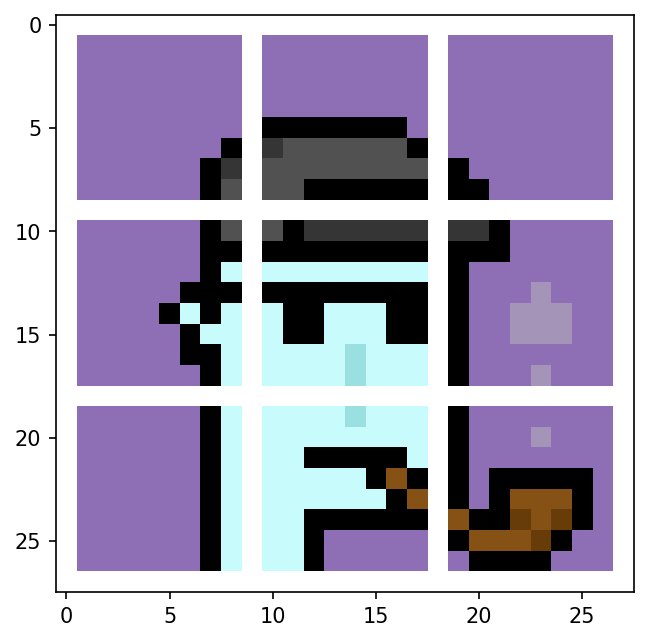
Block viewing is mportant for understanding ubiquitous image and video compression schemes like JPEG

Here we consider an image as a grid of non-overlapping blocks, each block containing a number of pixels. A block transform is where we replace each block from the original image with a block of our choosing. We could choose to replace the whole collection of pixels in a block with the average or median color of the block.

The compression schemes we will be soon learning about rely on spatial coherence to consider each block as a collection of characteristics (mean, differences, whatever) rather than as a collection if independent pixels. Depending on the descriptive power of any particular characteristic, we may choose to heavily quantize or even ignore that characteristic in order to save space, leading to a lossy compression that does not badly affect the perceived image quality.

Imports¶

We add several functions from the skimage module:

view_as_blocks decomoposes an image into blocks of a defined size.
montage allows us to reassemble a bunch of blocks back into a grid.
We use resize or rescale to ensure that our image and glyphs have a common denominator that we can use as a block size.

%matplotlib inline
import matplotlib.pyplot as plt
import numpy as np

import skimage.color as color

# For importing from alternative directory sources
import sys  
sys.path.insert(0, '../dip_utils')

from matrix_utils import (arr_info,
                          make_linmap)
from vis_utils import (vis_rgb_cube,
                       vis_hists,
                       vis_pair)

from skimage.util import view_as_blocks
from skimage.util import montage
from skimage.transform import resize, rescale

Load a small image¶

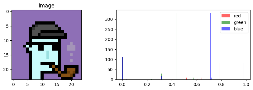
We’re using one with a resolution that is a multiple of 8, since we’d like to use 8x8 blocks. This cryptopunk7804 is sourced from a non-fungible token (NFT) that was recently valued at $\sim\$16M$ , though that could be from wash trading.

I = plt.imread('../dip_pics/cryptopunk7804.png')
I = I[...,:3] # cut out the alpha channel
vis_hists(I)
print(arr_info(I))

((24, 24, 3), dtype('float32'), np.float32(0.0), np.float32(0.9843137))

View as Blocks¶

You can see the above is a $24x24x3$ array of floats in $[0,1]$ . view_as_blocks will allow us to consider this image as a grid of non-overlapping $8x8x3$ blocks. (Remember the 3 is the R-G-B axis.)

block_shape = (8,8,3)

view = view_as_blocks(I, block_shape)
arr_info(view)

((3, 3, 1, 8, 8, 3), dtype('float32'), np.float32(0.0), np.float32(0.9843137))

As you can see, the resulting view variable is a $3x3$ grid of these $8x8x3$ blocks. Let’s consider it as a linear list of blocks instead of a grid. When we reshape we have to be careful to maintain the $8x8x3$ elements of this list.

block_view = np.reshape(view, [view.shape[0]*view.shape[1]] + list(block_shape))
arr_info(block_view)

((9, 8, 8, 3), dtype('float32'), np.float32(0.0), np.float32(0.9843137))

Montage¶

We can use montage to reassemble the block_view into a single displayable image again. We’ll add padding so that you can see the decomposition into blocks.

I_block_grid = montage(block_view, grid_shape=view.shape[:2], channel_axis=-1, padding_width=1, fill=[1,1,1])

plt.figure(figsize=(5,5))
plt.imshow(I_block_grid)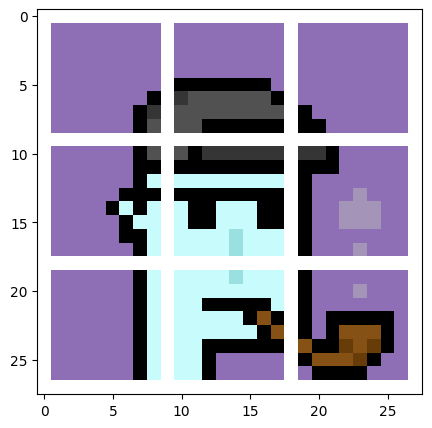

Transforming or Processing Blocks¶

With this block_view we can even even apply some kind of transform or function to each block, computing some block characteristics. Here, we’ll replace each block with its mean color. We’ll make a new list of blocks and then put our modified blocks into it, so that we can montage the modified image later.

mod_block_view = np.zeros_like(block_view)

for i, block in enumerate(block_view):
    block_mean = block.mean(axis=(0,1)) # Get the average color in the block.
    
    # Here we're setting all pixels in the block to the average color.
    # This works because block_mean has shape (3,) and block has shape (8,8,3),
    # so broadcasting applies.
    mod_block_view[i] = block_mean

mod_block_grid = montage(mod_block_view, grid_shape=view.shape[:2], channel_axis=-1, padding_width=1, fill=[1,1,1])

plt.figure(figsize=(5,5))
plt.imshow(mod_block_grid)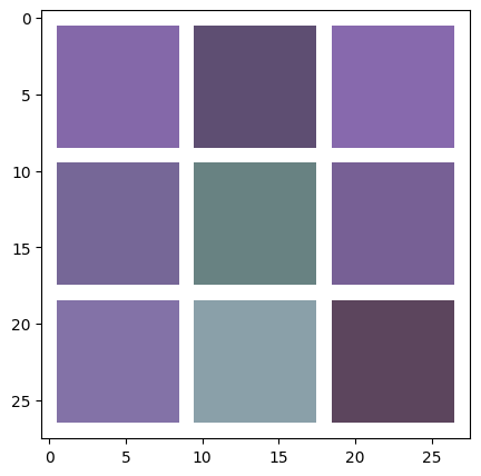

In this particular example we’ve processed a $24x24$ image into a $3x3$ . With only 9 pixels of course, the image is pretty poorly resolved, but we have in a sense compressed the image 64-fold (a factor of 8 in $x$ and 8 in $y$ ).

🔨 Your Turn: Block Means on a Larger Image¶

A $24 \times 24$ image is good for seeing every block, but it hides how well (or badly) this works on a real photograph.

Task: Apply the same mean-per-block decomposition to a larger image of your choosing, with $8 \times 8$ blocks, and show the original and block-mean versions side by side. Then try $4 \times 4$ and $16 \times 16$ blocks. At what block size does the image stop being recognizable?

Guidance:

You have to be careful that the block size you choose evenly divides the shape of the image itself. Either crop the image so that its height and width are multiples of the block size, or resize it.
Check the image with arr_info first. .png files may have a fourth (alpha) channel to remove, as we did above.
Reassemble with montage, but leave out the padding this time (or the white lines will dominate a large image), so you can compare with vis_pair and zoom into the same region of both.
How many numbers does the block-mean version need, compared with the original?

🔨 Your Turn: Keeping More Information per Block¶

In the above, every $8 \times 8$ block is characterized by a single color, the average of the block. If you could keep any additional information about it, even at the cost of maybe being less compressive, what additional information might you keep?

Task: Try keeping four averages in each block. That is, consider the block as four quarters and store the mean color of each quarter. Show the result next to the one-mean-per-block version. This will be no doubt a better representation of the original, though at what cost?

Guidance:

Each $8 \times 8$ block has four $4 \times 4$ quarters, which you can reach by slicing the block. Fill each quarter of the modified block with that quarter’s mean color.
Note: a block size of $4 \times 4$ would accomplish the same thing. Use that to check your result.
Count the numbers stored per block in each version, to describe the cost.

🧠 Further Efforts¶

Here are some other block-based techniques you could explore on a larger image of your choosing.

Median color per block. Instead of the mean, compute the median color of each block, channel by channel. Compare it with the mean at a block boundary that crosses a strong edge. Which keeps edges crisper, and why?
Guidance: np.median takes an axis argument just as mean does. Look at a block that is mostly one color with a few pixels of another.
Measure activity per block. Along with the mean color, compute a measure of how busy each block is, such as its standard deviation (compare the local standard deviation in the non-linear filtering demo). Display the activity of every block as a small image. Which blocks would a smart compression scheme spend more bits on?
Guidance: Compute the activity on a grayscale version of the image, so that each block gets a single number.
Dominant colors per block. Use k-means with $K = 2$ on the pixels of each block to find its two most representative colors, and replace every pixel with the closer of the two. How does it compare with the four-quarters version, which also stores more than one color per block?
Guidance: scipy.cluster.vq.kmeans2 works on an $N \times 3$ array of a block’s pixels. Some blocks are a single flat color; make sure your code copes.
Multiple scales. Compute block means at $32 \times 32$ , $16 \times 16$ , and $8 \times 8$ , and then store each finer level only as its difference from the coarser level above it. Why are those differences small for most blocks?
Guidance: This is the idea behind progressive image formats that load as a blurry image that sharpens, and behind Haar wavelets. Look at the histograms of the differences.