Comparing Reconstruction Efficiency - imageprocessing-awesome

Standard, Random, Haar, DCT, and the Karhunen-Loève Transform¶

DRAFT, not finalized. This chapter is new and still under review.

stough 202-

Preview: Comparing Reconstruction Efficiency

Blocks as vectors, bases as matrices
Reconstructing from a few coefficients
Why the error is the energy we dropped: Parseval
The Karhunen-Loève transform
The comparison
The KLT looks like the DCT
Why JPEG chose the DCT
🔨 Your Turn: Beat the DCT
🧠 Further Efforts

Throughout this chapter we’ve described $8 \times 8$ image blocks in different bases: the standard basis (one coefficient per pixel), Haar wavelets, the DCT, even a random one. Each is a complete, orthonormal basis, so each represents every block exactly. They differ in how efficiently they do it: how much of the block they capture with only a few coefficients. That’s what decides how well a basis compresses.

In this notebook we’ll put a number on that efficiency for every basis, on real images, and add one more basis: the Karhunen-Loève transform (KLT), the basis that is provably the most efficient for a given image. Then we’ll see why JPEG nonetheless uses the DCT.

We’ll reconstruct images from a few coefficients in each basis, measure the error, and then see, through a theorem of Parseval’s, why the error comes out the way it does.

%matplotlib inline
import matplotlib.pyplot as plt
import numpy as np
from skimage.color import rgb2gray
from skimage.util import view_as_blocks

# For importing from alternative directory sources
import sys
sys.path.insert(0, '../dip_utils')

from matrix_utils import arr_info
from vis_utils import vis_triple
from wavelet_utils import (make_haar_matrix,
                           make_random_basis,
                           make_klt_basis,
                           make_dct_matrix,
                           make_standard_matrix)

Blocks as Vectors, Bases as Matrices¶

So far we’ve transformed a block $\mathbf{B}$ with a $2D$ product, $\mathbf{T} = \mathbf{H}\mathbf{B}\mathbf{H}^\intercal$ . For comparing bases, it’s more convenient to flatten each $8 \times 8$ block into a vector $\mathbf{b}$ of 64 numbers. Then any basis of $8 \times 8$ patterns is a $64 \times 64$ orthonormal matrix $\mathbf{K}$ whose rows are the flattened patterns, and the transform is a single matrix-vector product:

\mathbf{c} = \mathbf{K}\mathbf{b}, \qquad \mathbf{b} = \mathbf{K}^\intercal\mathbf{c}.

For the bases built from an $8 \times 8$ matrix $\mathbf{H}$ , the 64 patterns are the outer products of pairs of rows of $\mathbf{H}$ (as vis_blocks shows), and $\mathbf{K}$ is the Kronecker product $\mathbf{H} \otimes \mathbf{H}$ . Let’s check that it agrees with $\mathbf{H}\mathbf{B}\mathbf{H}^\intercal$ on a random block.

H = make_dct_matrix(8)
K = np.kron(H, H)                         # 64 x 64
print(arr_info(K))

B = np.random.random((8, 8))
print('agrees with H B H^T:', np.allclose(K @ B.ravel(), (H @ B @ H.T).ravel()))
print('orthonormal:', np.allclose(K @ K.T, np.eye(64)))

((64, 64), dtype('float64'), np.float64(-0.24048494156391095), np.float64(0.24048494156391095))
agrees with H B H^T: True
orthonormal: True

Now an image becomes a matrix $\mathbf{X}$ with one flattened block per row, and the coefficients of every block in basis $\mathbf{K}$ are the rows of $\mathbf{C} = \mathbf{X}\mathbf{K}^\intercal$ . We’ll work in grayscale, with a few test images from dip_pics, cropped so that the blocks fit.

def load_gray(name):
    I = plt.imread('../dip_pics/' + name)
    I = rgb2gray(I[..., :3]) if I.ndim == 3 else I
    I = I.astype(float)
    I = I / 255 if I.max() > 1 else I
    return I[:I.shape[0] // 8 * 8, :I.shape[1] // 8 * 8]     # crop to whole blocks

def to_blocks(I):
    '''An N x 64 matrix: one flattened 8x8 block per row.'''
    return view_as_blocks(I, (8, 8)).reshape(-1, 64)

names = ['peppers.png', 'mountainSpring.jpg', 'girl_with_glasses.png', 'roadforest.jpg']
images = {name: load_gray(name) for name in names}

fig, ax = plt.subplots(1, 4, figsize=(12, 2.6))
for a, name in zip(ax, names):
    a.imshow(images[name], cmap='gray', vmin=0, vmax=1)
    a.set_title(f'{name}\n{to_blocks(images[name]).shape[0]} blocks', fontsize=9)
    a.set_axis_off()
plt.tight_layout()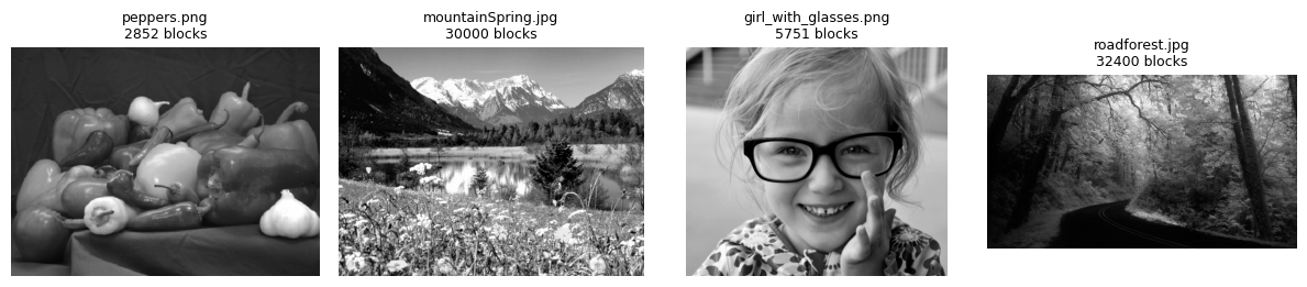

Reconstructing from a Few Coefficients¶

To compress, we keep only some of each block’s 64 coefficients, set the rest to zero, and reconstruct with $\hat{\mathbf{b}} = \mathbf{K}^\intercal\hat{\mathbf{c}}$ . Which coefficients should we keep? To compare bases fairly, we’ll use zonal selection: for each basis, find the $k$ coefficient positions that have the most energy on average over all the blocks of the image, and keep those same $k$ positions in every block.

Then we put the reconstructed blocks back together into an image and compare it with the original. Our measure is the PSNR, computed from the mean squared difference between the two images.

def to_image(Xb, shape):
    '''Reassemble an N x 64 matrix of flattened blocks into an image of the given shape.'''
    h, w = shape
    return Xb.reshape(h // 8, w // 8, 8, 8).transpose(0, 2, 1, 3).reshape(h, w)

def zonal_positions(C):
    '''Coefficient positions ordered by average energy over all blocks, largest first.'''
    return np.argsort((C**2).mean(axis=0))[::-1]

def reconstruct(I, K, k):
    '''Reconstruct image I keeping, in every block, the k most energetic positions of basis K.'''
    X = to_blocks(I)
    C = X @ K.T                                  # coefficients of every block
    keep = zonal_positions(C)[:k]
    C_kept = np.zeros_like(C)
    C_kept[:, keep] = C[:, keep]                 # zero all but the kept positions
    return to_image(C_kept @ K, I.shape)         # b = K^T c for every block (as rows: c^T K)

def psnr(I, J):
    return 10 * np.log10(1 / np.mean((I - J)**2))

I = images['peppers.png']
print('to_image undoes to_blocks:', np.array_equal(to_image(to_blocks(I), I.shape), I))

K_dct = np.kron(make_dct_matrix(8), make_dct_matrix(8))
R = reconstruct(I, K_dct, 8)
vis_triple(I, np.clip(R, 0, 1), I - R, cmap='gray', figsize=(11, 3), show_ticks=False,
           first_title='original', second_title=f'DCT, 8 of 64 kept: {psnr(I, R):.1f} dB',
           third_title='difference (original - reconstruction)')

to_image undoes to_blocks: True

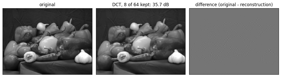
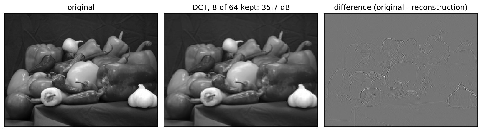
reconstruct follows the steps exactly: cut the image into blocks, transform every block, keep the $k$ most energetic positions, transform back, and reassemble. Since the blocks are rows of X, transforming all of them at once is X @ K.T, and transforming back is C_kept @ K. to_image undoes to_blocks, as the printed check confirms.

Keeping only 8 of each block’s 64 DCT coefficients, an 8-fold reduction, the reconstruction is hard to tell from the original at this size. The difference image (right) shows what was lost: it’s flat gray (zero) in smooth regions, and the error concentrates along edges, tracing the outlines of the peppers and the garlic. Zoom in on the reconstruction to see the slight blur there.

Why the Error Is the Energy We Dropped: Parseval¶

There’s a neat way to predict that error without reconstructing anything. Because $\mathbf{K}$ is orthonormal, it preserves lengths: $\|\mathbf{K}\mathbf{v}\| = \|\mathbf{v}\|$ for every vector $\mathbf{v}$ . (Rotations and reflections in 64 dimensions, just like in 2.) This is Parseval’s theorem. Apply it to the error vector of a block: the error in the pixels has exactly the same energy as the error in the coefficients, and the error in the coefficients is just the coefficients we dropped. So

\|\mathbf{b} - \hat{\mathbf{b}}\|^2 = \sum_{\text{dropped } j} c_j^2.

Averaged over the blocks and divided by 64, the dropped energy is the mean squared error. Let’s check that against the error we just computed by reconstructing.

C = to_blocks(I) @ K_dct.T
dropped = zonal_positions(C)[8:]                          # every position but the 8 kept ones
mse_parseval = (C[:, dropped]**2).mean(axis=0).sum() / 64
mse_computed = np.mean((I - R)**2)
print(f'MSE from reconstructing: {mse_computed:.3e}')
print(f'MSE from Parseval:       {mse_parseval:.3e}')

MSE from reconstructing: 2.678e-04
MSE from Parseval:       2.678e-04

The same number both ways. This is why energy compaction is the right way to judge a basis for compression: whatever energy a basis packs into the coefficients we keep is energy that can’t show up as error. A basis that puts most of a block’s energy into a few coefficients will reconstruct it well from those few.

The Karhunen-Loève Transform¶

That suggests a question: which orthonormal basis would pack the most energy into its first $k$ coefficients, on average over the blocks? We want the first basis vector to capture as much of the blocks’ energy as possible, the second as much of what remains, and so on. That is exactly the question that principal component analysis answers: the best directions are the eigenvectors of the blocks’ second-moment matrix $\frac{1}{N}\mathbf{X}^\intercal\mathbf{X}$ , in order of decreasing eigenvalue. In compression, this basis is called the Karhunen-Loève transform, and no other basis does better at zonal coding of the image it was computed from.

We’ll compute the full 64-dimensional KLT from the blocks. wavelet_utils also has make_klt_basis, which computes a cheaper separable version from 8-pixel runs, to be used like the other $8 \times 8$ matrices; we’ll include it too.

def klt_basis(X):
    '''64 x 64 KLT for blocks X: eigenvectors of the second-moment matrix, largest eigenvalue first.'''
    vals, vecs = np.linalg.eigh(X.T @ X / X.shape[0])     # eigh: for symmetric matrices, sorted ascending
    return vecs[:, ::-1].T                                # rows are basis vectors, most energetic first

K_klt = klt_basis(to_blocks(I))
print('orthonormal:', np.allclose(K_klt @ K_klt.T, np.eye(64)))

orthonormal: True

The Comparison¶

Here are all the bases on the peppers image, first by eye, keeping 8 coefficients per block. make_random_basis gives a different random basis each time; any one is as good (or bad) as another.

bases = {
    'standard':       np.kron(make_standard_matrix(8), make_standard_matrix(8)),
    'random':         np.kron(make_random_basis(8), make_random_basis(8)),
    'Haar':           np.kron(make_haar_matrix(8), make_haar_matrix(8)),
    'DCT':            K_dct,
    'separable KLT':  np.kron(make_klt_basis(I, 8), make_klt_basis(I, 8)),
    'KLT':            K_klt,
}

plt.ion()
fig, ax = plt.subplots(2, 6, figsize=(14, 4.2), sharex=True, sharey=True)
for col, (name, K) in enumerate(bases.items()):
    R = reconstruct(I, K, 8)
    ax[0, col].imshow(np.clip(R, 0, 1), cmap='gray', vmin=0, vmax=1)
    ax[0, col].set_title(f'{name}: {psnr(I, R):.1f} dB', fontsize=9)
    ax[1, col].imshow(I - R, cmap='gray', vmin=-0.25, vmax=0.25)
for a in ax.flat:
    a.set_axis_off()
ax[1, 0].set_title('differences (same scale)', fontsize=9, loc='left')
plt.tight_layout()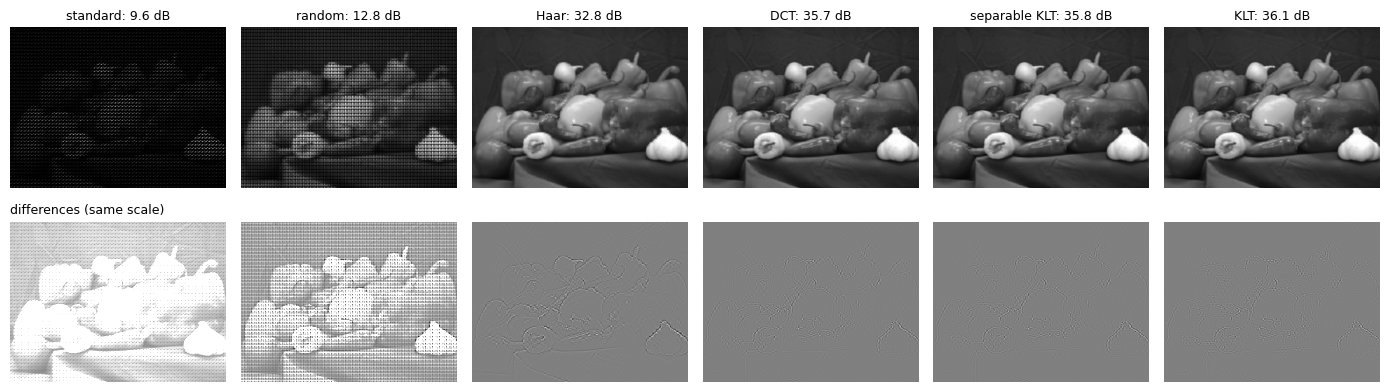

Each column is one basis, with its reconstruction from 8 of 64 coefficients per block on top and the difference from the original below, all on the same gray scale (mid-gray is zero error).

The standard basis keeps 8 pixels of every block and zeroes the other 56, so most of the image is simply black, and the difference image is the image itself. The random basis does little better: every random pattern carries about the same share of the energy, so there are no coefficients that can be safely dropped.
Haar looks good at this size too, but its difference image shows clearly stronger errors along every edge, and zooming in on the reconstruction shows its blocks.
The DCT, the separable KLT and the KLT are nearly indistinguishable, with the smallest and most edge-confined differences.

To see the whole range of compression, here’s the PSNR as a function of the number of coefficients kept, each point computed by reconstructing the image as above.

ks = np.arange(1, 64)            # at k = 64 every basis is exact and the PSNR is infinite
fig, ax = plt.subplots(figsize=(7, 4))
for name, K in bases.items():
    curve = [psnr(I, reconstruct(I, K, k)) for k in ks]
    ax.plot(ks, curve, label=name, lw=2 if 'KLT' in name or name == 'DCT' else 1)
ax.set_xlabel('coefficients kept per block (of 64)')
ax.set_ylabel('PSNR (dB)')
ax.set_title('peppers.png')
ax.set_xscale('log', base=2)
ax.grid(alpha=0.3)
ax.legend();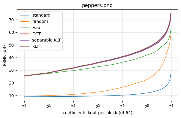

Higher is better, and the $k$ axis is on a log scale: 1, 2, 4, ... 32 coefficients. The ranking from the images holds all the way along. The standard and random bases improve only slowly. Haar is far better, since its patterns are made to exploit spatial coherence. And the DCT is better still, nearly indistinguishable from the KLT, the best possible.

To read it as compression: at 8 coefficients per block, the DCT and KLT reach about 36 dB, about 2.5 dB above Haar and more than 25 dB above the standard basis. Every 10 dB is a factor of 10 in mean squared error, so that’s hundreds of times less error than keeping 8 of the 64 pixels.

But the KLT here had an advantage: it was computed from the peppers themselves. What if we use a KLT computed from a different image? Let’s tabulate the PSNR at 8 coefficients per block for every image, with the DCT, the image’s own KLT, and a KLT computed from the mountain photo.

K_mountain = klt_basis(to_blocks(images['mountainSpring.jpg']))

print(f"{'image':24s} {'DCT':>7s} {'own KLT':>9s} {'mountain KLT':>13s}")
for name in names:
    Ii = images[name]
    own = klt_basis(to_blocks(Ii))
    print(f'{name:24s} {psnr(Ii, reconstruct(Ii, K_dct, 8)):7.2f} {psnr(Ii, reconstruct(Ii, own, 8)):9.2f} '
          f'{psnr(Ii, reconstruct(Ii, K_mountain, 8)):13.2f}')

image                        DCT   own KLT  mountain KLT
peppers.png                35.72     36.07         35.33

mountainSpring.jpg         23.22     23.29         23.29
girl_with_glasses.png      33.20     33.46         33.23

roadforest.jpg             28.39     28.56         28.45

On every image, the image’s own KLT is the best (in the mountain row, the own KLT and the mountain KLT are the same basis). But the DCT is within a few tenths of a dB of it every time. And a KLT borrowed from another image is about as good as the DCT: a few hundredths of a dB better on some images, and on the peppers almost 0.4 dB worse. The KLT’s advantage is real but tiny, and it doesn’t travel.

The KLT Looks Like the DCT¶

Why is the DCT so close to optimal? Let’s look at the KLT’s basis patterns, the rows of K_klt reshaped to $8 \times 8$ , next to the DCT’s, both sorted by how much energy they capture on the peppers.

def show_patterns(K, X, ax, title, n=16):
    order = np.argsort(((X @ K.T)**2).mean(axis=0))[::-1]   # most energetic first
    for a, j in zip(ax.flat, order[:n]):
        P = K[j].reshape(8, 8)
        a.imshow(P, cmap='gray', vmin=-np.abs(P).max(), vmax=np.abs(P).max())
        a.set_xticks([])      # no ticks, but keep the frame, so a flat pattern is still visible
        a.set_yticks([])
    ax.flat[0].set_title(title, loc='left', fontsize=10)

fig, ax = plt.subplots(2, 8, figsize=(10, 2.8))
X = to_blocks(I)
show_patterns(K_dct, X, ax[0], 'DCT, 8 most energetic', n=8)
show_patterns(K_klt, X, ax[1], 'KLT of the peppers, 8 most energetic', n=8)
plt.tight_layout()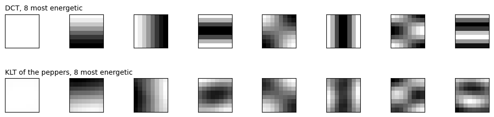

Strikingly similar patterns, at least up to sign: a flat block first, then gentle ramps in each direction, then finer cosine-like waves. Computed from nothing but the data, the KLT has nearly rediscovered the DCT. The match isn’t exact: the KLT’s patterns are a little irregular, and by the seventh and eighth they begin to drift apart, but those later patterns carry little of the energy.

This isn’t a coincidence. If neighboring pixels are strongly correlated, with the correlation falling off with distance, as it is in essentially all natural images, then the KLT tends toward the DCT as the correlation approaches 1. That is the mathematical content of spatial coherence: the DCT is the KLT of the generic natural image.

Why JPEG Chose the DCT¶

Putting it together, the DCT was the natural choice for the JPEG standard:

Nearly optimal. On natural images it comes within a fraction of a dB of each image’s own KLT, as we saw.
Fixed. The KLT depends on the image, so an encoder would have to compute it for every image and send the $64 \times 64$ basis along with it. The DCT is known in advance by every encoder and decoder.
Fast. Like the Fourier transform, to which it’s closely related, the DCT has fast algorithms; and since it’s separable, the 2D transform is just 1D transforms of the rows and columns. A general $64 \times 64$ KLT is a full matrix multiply per block.

The KLT remains important as a benchmark, the best that any linear transform can do, and in settings where the data are unusual and a basis can be learned once and reused, such as the face spaces of the PCA chapter.

🔨 Your Turn: Beat the DCT¶

The DCT came within a fraction of a dB of the KLT on all of our test images. Is that always true?

Task: Find or make an image on which the image’s own KLT beats the DCT by at least 1 dB at 8 coefficients per block. Show the image, the two PSNR values, and the two sets of most-energetic patterns. Explain what about your image makes the DCT a poor fit.

Guidance:

Think about what assumption makes the DCT nearly optimal: smooth, spatially coherent content, correlated in every direction, with no preferred pattern. What kinds of images break that?
Photographs rarely do. Even textures like skimage.data.brick() or data.text() get within about half a dB. You’ll probably need a synthetic image built with NumPy: think about an image whose blocks are all alike, or nearly alike, in a way that isn’t smooth.
load_gray, to_blocks, reconstruct, psnr, klt_basis, and show_patterns above work on any grayscale image in $[0, 1]$ , as long as its sides are multiples of 8.
Looking at the KLT’s patterns for your image is the best way to understand why it wins.

🧠 Further Efforts¶

Adaptive selection. We kept the same $k$ positions in every block (zonal coding). Instead, keep each block’s own $k$ largest coefficients, as the Haar exercise asks. Compare the PSNR curves for each basis with the zonal ones. How much does adaptivity help each basis, and does it change their ranking? Check one of your PSNRs with Parseval.
Guidance: The selection now differs from block to block, so build a mask the same shape as C rather than a single list of positions. Keep in mind that adaptive selection costs extra bits in practice, to record which positions each block kept.
Block size. Repeat the comparison with $4 \times 4$ and $16 \times 16$ blocks, at the same compression ratio (keeping 1/8 of the coefficients). Which block size works best for the DCT, and why might JPEG have settled on $8 \times 8$ ?
Guidance: make_dct_matrix, make_haar_matrix, and view_as_blocks all take the size as a parameter; the KLT for $16 \times 16$ blocks is $256 \times 256$ .
Color. For a color image, compare transforming the R, G, and B channels with transforming the Y, Cb, and Cr channels of YCbCr. Where does the energy go in each case?
Guidance: Compute the total energy of each channel’s coefficients, and the PSNR of each channel at 8 coefficients per block.