Haar Compression Activity

stough 202-

DIP 6, 8.9

In this activity you’re going to use the Haar wavelet block transform and lossy compression in two different contexts

A single $4x4$ single-channel “image” block with fairly high contrast.
A larger color image with $8x8$ blocks.

In each case we’re going to

Transform: Turn a block of image pixels into a block of Haar wavelet coefficients.
Compress: We’re going to effectively compress by zeroing out insigficant/small coefficients.
Reconstruct: Take the “compressed” coefficent block and reconstruct the block of image pixels, with some loss.

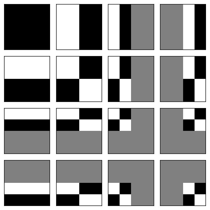
Recall from view_basis_blocks that the Haar $4x4$ transform matrix is like so:

\mathbf{H_{Haar}} = \frac{1}{2}\begin{vmatrix} 1 & 1 & 1 & 1\\ 1 & 1 & -1 & -1 \\ {\sqrt 2} & -{\sqrt 2} & 0 & 0 \\ 0 & 0 & {\sqrt 2} & -{\sqrt 2} \end{vmatrix}

To transform a block of pixels $\mathbf{B}$ into a block of coefficients $\mathbf{T}$ :

\mathbf{T} = \mathbf{H}\times\mathbf{B}\times\mathbf{H}^T

where $\mathbf{H}^T$ is the transpose. Through the above we basically replace the set of independent pixels with the set of coefficients with respect to the Haar basis patterns, as we’ll see with vis_blocks. Once we have $\mathbf{T}$ , we can quantize it to the degree that we wish, zeroing out small coefficients, potentially replacing large coefficients with nearby approximations on a standard grade (e.g. replace anything in $[236,276]$ with 256).

To reconstruct the original $\mathbf{B}$ , we can simply

\mathbf{B} = \mathbf{H}^T\times\mathbf{T}\times\mathbf{H}

Imports¶

We’re going to use wavelet_utils.

%matplotlib inline
import matplotlib.pyplot as plt
import numpy as np

# For importing from alternative directory sources
import sys  
sys.path.insert(0, '../dip_utils')

from matrix_utils import (arr_info,
                          make_linmap)
from vis_utils import (vis_rgb_cube,
                       vis_hists,
                       vis_pair,
                       vis_triple,
                       vis_surface)

from wavelet_utils import (make_haar_matrix,
                           make_random_basis,
                           make_klt_basis,
                           make_dct_matrix,
                           make_standard_matrix,
                           vis_blocks)

1. $4\times4$ Haar Wavelet Compression¶

Use make_haar_matrix and vis_blocks to see the 16 Haar patterns for the $\mathbf{H_{Haar}}$ matrix.

The function vis_blocks shows all possible outer products of rows in the input matrix. If the $N\times N$ input is a transform matrix $\mathbf{H}$ (whose rows are all orthogonal to one another, unit length, spanning the $N$ -D space), then vis_blocks shows the collection of $N\times N$ patterns that the transform matrix implies.

H = make_haar_matrix(4)
vis_blocks(H)

Transform a $4\times4$ block of pixels.¶

We’ll define the block of pixels in question. Then you transform it into the coefficient block $\mathbf{T}$ . See np.matmul to compute $\mathbf{H}\times\mathbf{B}\times\mathbf{H}^T$ . You can think of $\mathbf{B}$ as a little patch of an image.

B = np.array([[0,1,1,1],
              [0,1,0,0],
              [0,1,1,1],
              [0,1,0,0]])

plt.figure(figsize=(4,4))
plt.imshow(B, cmap='gray')

A. Viewing the transform coefficients in the matrix $\mathbf{T}$ , what are the row and column coords for the two largest coefficients (in absolute value)?¶

Do not view $\mathbf{T}$ with vis_blocks. $\mathbf{T}$ is not a transform matrix; it is a matrix of coefficients, each coefficient corresponding to one of the patterns that you saw with vis_blocks(H) for a given transform matrix $\mathbf{H}$ .

B. Show the two basis blocks corresponding to those two coefficients.¶

C. Show and explain as explicitly as you can how the two coefficients are what they are.¶

D. Show the reconstruction of the image $\mathbf{B}$ using only those basis blocks/coefficients.¶

Is this reconstruction trending in the right direction? Explain.

2. Larger Image Block Transform and Reconstruction.¶

Use the code in block_viewing_demo and basis_decomp_64pix to perform a similar transform/compress/reconstruct sequence on a larger color image of your choice.

Use $8\times8\times3$ blocks. However, you should process each color channel separately.
Use resize on the image you choose to ensure that 8 evenly divides it in height and width. This is for convenience: compression schemes have other mechanisms to deal with odd-shaped images, which we will ignore here.
Perform reconstructions using the largest $[1,2,4,8,16]$ coefficients in absolute value per block. Note that keeping 16 coefficients for example is equivalent to $\sim 4$ x compression -- that is, moving from storing 64 pixel values to storing 16 coefficient values.
For each $k$ coefficient visualization, you should keep $k$ coefficients per color channel. So for example with 1 coefficient, that’s 1 red, 1 blue, 1 green.
For at least the reconstructions using $[2,4]$ , use vis_pair and zoom into an area to observe the effectiveness of the reconstruction on such limited basis (32x, 16x compression). Use vis_triple for example to view the original image along with these lossy reconstructions.

Imports¶

1. 4×44\times44×4 Haar Wavelet Compression¶

Transform a 4×44\times44×4 block of pixels.¶

A. Viewing the transform coefficients in the matrix T\mathbf{T}T, what are the row and column coords for the two largest coefficients (in absolute value)?¶