Basis and reconstruction of 64 pixel image.

stough 202-

DIP

Decompose and partially reconstruct according to the Haar basis.

If we think of an image as a collection of independent pixels, then the only way to describe an image would be “the first pixel’s color is x, the second pixel’s color is y, ...” However, you would never describe an image like that, and spatial coherency states that neighboring pixels are usually closely related in color. Rather than think of an image as a collection pixels, in this demo we reimagine the image as a collection of patterns, where we simply mix how much of each pattern we need.

This is an application of a change of basis in linear algebra.

%matplotlib inline
import matplotlib.pyplot as plt
import numpy as np

# For importing from alternative directory sources
import sys  
sys.path.insert(0, '../dip_utils')

from matrix_utils import (arr_info,
                          make_linmap)
from vis_utils import (vis_rgb_cube,
                       vis_hists,
                       vis_pair)

from wavelet_utils import (make_haar_matrix,
                           make_random_basis,
                           make_klt_basis,
                           make_dct_matrix,
                           make_standard_matrix)

print('haarReconstructionDemo: Works only on 64 pixel images...')

I = plt.imread('../dip_pics/surprise.png')
# I = plt.imread('strawberry.png')


H = make_haar_matrix(8)

#The transform image, an image of coefficients wrt the Haar basis.
CT = np.zeros(I.shape)
for chan in range(3):
    CT[...,chan] = np.matmul(H, np.matmul(I[...,chan], H.transpose()))


#RI will represent the reconstructed image as we add back more
#Haar patterns
RI = np.zeros(I.shape) #Still should be 8x8


#Visual
fh, axh = plt.subplots(8,8, figsize=(8,8), num='Haar Basis Images and Coefficients')
fr, axr = plt.subplots(8,8, figsize=(8,8), num='Partial Reconstructions from Large Scale to Small')


# We're going to reconstruct according to distance from the
# 0,0 (the first Haar basis, average calculator). Notice,
# this order is independent of the actual image data.
xs = np.meshgrid(np.arange(8), np.arange(8), indexing='ij')
coords = np.concatenate([np.expand_dims(c, axis=1) for c in
                         [x.ravel() for x in xs]], axis=1)
dists = np.sum(coords*coords, axis=1)
darg = np.argsort(dists) #sorts in increasing order
is_mags = False

#If we were to use magnitude of the coefficient...
# mags = CT[...,0].ravel(order='F')
# darg = np.argsort(np.abs(mags))
# darg = list(reversed(darg))
# is_mags = True

#
#c = 1 #used to display the order of reconstruction.

for which_axis, which_basis in enumerate(darg):
    i,j = coords[which_basis] #coords[darg[x]] if x in range(len(darg))
    
    wa_i = i
    wa_j = j
    
    if is_mags:
        wa_i = which_axis//8
        wa_j = which_axis%8

    #Construct that Haar basis and display it
    Bij = np.outer(H[i, :], H[j, :])
    axh[wa_i][wa_j].imshow(Bij, cmap='gray', vmin=-.5, vmax=.5)
    axh[wa_i][wa_j].axes.get_xaxis().set_visible(False)
    axh[wa_i][wa_j].axes.get_yaxis().set_visible(False)
    # axh[i][j].set_title('c_%d_%d: %6.3f' % (i, j, T[i,j]))
    # https://matplotlib.org/api/pyplot_api.html#matplotlib.pyplot.text
    axh[wa_i][wa_j].text(0, 6, r'$\pi:%6.3f$' % CT[i, j, :].sum(), fontsize=6, color='cyan')

    # Add the amount of that basis that was in the original image to
    # the running total, or reconstruction.
    # RI = RI + T[i, j] * Bij #2D
    for chan in range(3):
        RI[...,chan] += CT[i,j,chan]*Bij

    RIcopy = RI.copy().clip(0,1)
    axr[wa_i][wa_j].imshow(RIcopy)
    axr[wa_i][wa_j].axes.get_xaxis().set_visible(False)
    axr[wa_i][wa_j].axes.get_yaxis().set_visible(False)
    # axr[i][j].text(0, 6, '%d' % c, fontsize=10, color='cyan')
    #The order of reconstruction isn't that informative, but useful for debugging.
    #c += 1


plt.show()

# fh.canvas.set_window_title('Haar Basis Images and Coefficients')
fh.tight_layout()

# fr.canvas.set_window_title('Partial Reconstructions from Large Scale to Small')
fr.tight_layout()

haarReconstructionDemo: Works only on 64 pixel images...

What the figures show¶

The cell above takes an $8 \times 8$ RGB pixel-art image $\mathbf{I}$ and computes its 2D Haar transform, one channel at a time:

\mathbf{C} = \mathbf{H}\,\mathbf{I}\,\mathbf{H}^\intercal

where the rows of the $8 \times 8$ matrix $\mathbf{H}$ are the 1D Haar basis vectors (see view_basis_blocks). Each coefficient $C_{ij}$ says how much of one 2D basis image $\mathbf{B}_{ij} = \mathbf{h}_i \mathbf{h}_j^\intercal$ (the outer product of rows $i$ and $j$ of $\mathbf{H}$ ) is in the image. Because $\mathbf{H}$ is orthonormal, the original image is exactly the sum of all 64 basis images, each weighted by its coefficient:

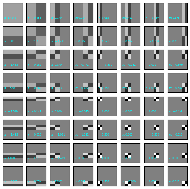
\mathbf{I} = \sum_{i=0}^{7} \sum_{j=0}^{7} C_{ij}\, \mathbf{B}_{ij}

The first figure shows the 64 basis images $\mathbf{B}_{ij}$ in their $(i,j)$ positions, with the coefficient (summed over the three color channels) printed in cyan. The top-left $\mathbf{B}_{00}$ is constant: its coefficient is proportional to the average color. Moving right or down, the patterns vary over smaller and smaller scales in the horizontal or vertical direction.
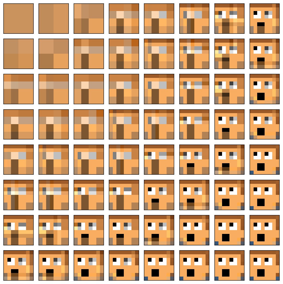
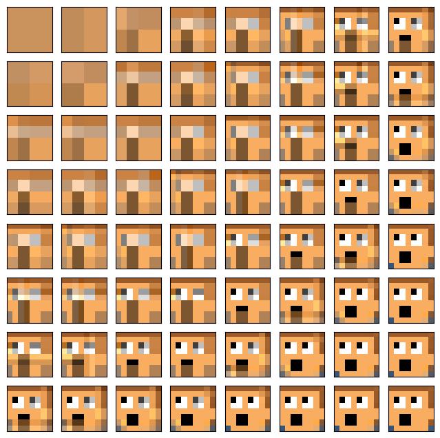
The second figure builds up the reconstruction by adding the basis images in order of distance from the top-left corner, roughly from coarse to fine scale. Panel $(i,j)$ shows the running sum after adding $C_{ij}\mathbf{B}_{ij}$ . The top-left panel is just the average color, and the image sharpens as you move toward the bottom-right panel, which is the exact original.

Notice how recognizable the face already is long before all 64 patterns have been added. Most of the image’s structure lives in the coarse patterns, and that observation is the foundation of transform coding.

🔨 Your Turn: Your Own Pixel Art, and Other Bases¶

Task:

Run the decomposition on your own $8 \times 8$ pixel art image. There are many examples out there, or maybe make your own.
Then try a different reconstruction basis. Update the line
```
H = make_haar_matrix(8)
```
and use an alternative like make_dct_matrix(8) or even make_random_basis(8). How does the order of reconstruction compare to Haar? How soon is the image recognizable?
Try the standard basis, make_standard_matrix(8). That’s the basis that says an image is a collection of pixels rather than a collection of patterns; it’s also called the Euclidean basis. Look at the coefficients that are reported in cyan. How are those coefficients distributed, versus when you use a pattern basis like Haar?

Guidance:

Copy the code cell above into the empty cell below, rather than editing it, so that you keep the Haar version to compare against.
The code works only on $8 \times 8$ RGB images with values in $[0,1]$ . Check yours with arr_info. Many downloaded “8×8” images are actually saved larger, with each art pixel drawn as a square of screen pixels; take every $k$ -th pixel to get back to $8 \times 8$ . Remove a fourth (alpha) channel if there is one.
All the bases in wavelet_utils are orthonormal ( $\mathbf{H}\mathbf{H}^\intercal = \mathbf{I}$ ), which is what makes the reconstruction exact. You can check that numerically for each one.
For the comparison, focus on the reconstruction figure: in each basis, how many of the 64 panels does it take before you would recognize the picture?