Haar Wavelets - imageprocessing-awesome

DRAFT, not finalized. This chapter is new and still under review.

stough 202-

From pixel pairs to a 1D transform
Repeating it: multiple levels
Two dimensions: the wavelet pyramid
Compression: keeping the largest coefficients
Interactive compression
Wavelets and JPEG 2000
🔨 Your Turn: Denoising by Shrinking Coefficients
🧠 Further Efforts

In Spatial Coherence and Change of Basis, we replaced each pair of neighboring pixels $\langle p_0, p_1 \rangle$ with their scaled sum and difference,

\begin{bmatrix} c_0 \\ c_1 \end{bmatrix} = \frac{1}{\sqrt2}\begin{bmatrix} 1 & 1 \\ 1 & -1 \end{bmatrix} \begin{bmatrix} p_0 \\ p_1 \end{bmatrix} = \frac{1}{\sqrt2}\begin{bmatrix} p_0 + p_1 \\ p_0 - p_1 \end{bmatrix},

and saw that because neighbors are similar, almost all of each pair’s energy lands in the “average” coefficient $c_0$ , while the “difference” $c_1$ is usually close to zero. Then in Viewing Basis Blocks and the 64-pixel decomposition we met the Haar basis as a matrix, make_haar_matrix, applied to $8 \times 8$ blocks.

This notebook connects the two. We’ll see that the Haar transform is nothing but that pixel-pair step, repeated, and that repeating it over a whole image gives a multi-scale picture of the image, the wavelet pyramid, in which most coefficients are nearly zero. That’s what makes wavelets so good for compression.

%matplotlib inline
import matplotlib.pyplot as plt
import numpy as np
from skimage.color import rgb2gray
from ipywidgets import VBox, FloatLogSlider

# For importing from alternative directory sources
import sys
sys.path.insert(0, '../dip_utils')

from matrix_utils import arr_info
from vis_utils import vis_pair
from wavelet_utils import make_haar_matrix

From Pixel Pairs to a 1D Transform¶

Take one row of an image. Split it into consecutive pairs, and replace every pair with its average and difference coefficients. Collect all the averages into one half-length signal, the approximation, and all the differences into another, the detail:

def haar_step_1d(x):
    '''One level of the 1D Haar transform along the last axis.
    Returns (approximation, detail), each half as long as x.'''
    even, odd = x[..., 0::2], x[..., 1::2]       # the first and second pixel of every pair
    return (even + odd) / np.sqrt(2), (even - odd) / np.sqrt(2)

I = rgb2gray(plt.imread('../dip_pics/peppers.png')[..., :3])
# Every level halves the image, so for up to 5 levels the height and width must be
# divisible by 2**5 = 32. Crop a little off the bottom and right to make it so.
I = I[:I.shape[0] // 32 * 32, :I.shape[1] // 32 * 32]
print(arr_info(I))

row = I[200]
approx, detail = haar_step_1d(row)

fig, ax = plt.subplots(3, 1, figsize=(8, 5), sharey=True)
ax[0].plot(row);            ax[0].set_title(f'row 200 of the image ({len(row)} pixels)')
ax[1].plot(approx / np.sqrt(2));   ax[1].set_title(f'approximation, scaled back by $1/\\sqrt{{2}}$ ({len(approx)} values)')
ax[2].plot(detail);         ax[2].set_title(f'detail ({len(detail)} values)')
plt.tight_layout()

((352, 480), dtype('float32'), np.float32(0.027428236), np.float32(0.99999994))

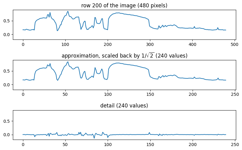
The x[..., 0::2] and x[..., 1::2] slices pick out the first and second pixel of every pair along the last axis, for every row at once if we pass in a whole image. Then the two sums are the average and difference, scaled by $1/\sqrt{2}$ to keep the transform orthonormal, as before.

The approximation (middle) is the row at half resolution: the same shape, with half as many samples. (It’s really $\sqrt{2}$ times the pair averages because of the normalization, so I’ve scaled it back for the plot.) The detail (bottom) is what the approximation lost: it hovers near zero, and only spikes where the row has a sharp edge, where two neighbors really differ. Together they hold exactly as many numbers as the row did, and the row can be recovered from them exactly: $p_0 = (c_0 + c_1)/\sqrt{2}$ and $p_1 = (c_0 - c_1)/\sqrt{2}$ .

Repeating It: Multiple Levels¶

The approximation is itself a signal with spatial coherence, so why stop? Apply the same step to the approximation, and again to the result, each time splitting off another detail signal at a coarser scale. After $L$ levels we have one small approximation and $L$ detail signals, from coarsest to finest:

x \;\to\; [\,a_1 \mid d_1\,] \;\to\; [\,a_2 \mid d_2 \mid d_1\,] \;\to\; [\,a_3 \mid d_3 \mid d_2 \mid d_1\,] \;\to\; \cdots

def haar_1d(x, levels):
    '''Multilevel 1D Haar transform: [approximation, coarsest detail, ..., finest detail].'''
    a, details = x, []
    for _ in range(levels):
        a, d = haar_step_1d(a)
        details.insert(0, d)            # coarser details go in front
    return np.concatenate([a] + details, axis=-1)

# For a signal of length 8, three levels take us all the way down to a single average.
x = np.array([4, 6, 10, 12, 8, 6, 5, 5], dtype=float)
H = make_haar_matrix(8)
print('repeated pair steps:', np.round(haar_1d(x, 3), 3))
print('H @ x:              ', np.round(H @ x, 3))

repeated pair steps: [19.799  2.828 -6.     2.    -1.414 -1.414  1.414  0.   ]
H @ x:               [19.799  2.828 -6.     2.    -1.414 -1.414  1.414  0.   ]

The two agree. The Haar matrix from make_haar_matrix is the pair step applied repeatedly, all the way down: its first row computes the overall average, the next row the coarsest difference (first half minus second half), and the later rows differences at finer and finer scales. The repeated-step version is also much faster: each level touches only half as many numbers as the one before, so the whole transform takes about $2N$ operations, compared with $N^2$ for multiplying by an $N \times N$ matrix.

Two Dimensions: The Wavelet Pyramid¶

For an image, we do one step along the rows and then one step down the columns. That splits the image into four quarter-size images, the subbands, as previewed at the end of intro_spatial_coherence:

top left: average along the rows and down the columns, a half-resolution copy of the image;
top right: difference along the rows (average down the columns), which responds to vertical edges;
bottom left: difference down the columns, which responds to horizontal edges;
bottom right: difference in both directions, for diagonal detail.

def haar_step_2d(I):
    '''One level of the 2D Haar transform: four subbands arranged in quadrants.'''
    a, d = haar_step_1d(I)                       # along the rows
    rows_done = np.concatenate([a, d], axis=1)
    a, d = haar_step_1d(rows_done.T)             # down the columns (transposed to the last axis)
    return np.concatenate([a, d], axis=1).T

def haar_2d(I, levels):
    '''Multilevel 2D Haar transform: repeat the step on the top-left (approximation) quadrant.'''
    C = I.astype(float).copy()
    h, w = C.shape
    for _ in range(levels):
        C[:h, :w] = haar_step_2d(C[:h, :w])
        h, w = h // 2, w // 2
    return C

def show_pyramid(C, levels, ax):
    '''Display a wavelet pyramid: the approximation as an image, details by magnitude.'''
    h, w = C.shape[0] >> levels, C.shape[1] >> levels
    is_detail = np.ones(C.shape, dtype=bool)
    is_detail[:h, :w] = False
    D = np.abs(C) / np.percentile(np.abs(C[is_detail]), 99)  # details: magnitude, top 1% saturated
    A = C[:h, :w]
    D[:h, :w] = (A - A.min()) / (A.max() - A.min())           # approximation: rescaled to [0, 1]
    ax.imshow(np.clip(D, 0, 1), cmap='gray')
    for k in range(levels):                                   # outline the quadrants
        hk, wk = C.shape[0] >> (k + 1), C.shape[1] >> (k + 1)
        ax.plot([wk, wk], [0, 2 * hk], 'r', lw=0.8)
        ax.plot([0, 2 * wk], [hk, hk], 'r', lw=0.8)
    ax.set_axis_off()

fig, ax = plt.subplots(1, 3, figsize=(11, 3))
ax[0].imshow(I, cmap='gray'); ax[0].set_axis_off(); ax[0].set_title('image')
show_pyramid(haar_2d(I, 1), 1, ax[1]); ax[1].set_title('one level')
show_pyramid(haar_2d(I, 3), 3, ax[2]); ax[2].set_title('three levels')
plt.tight_layout()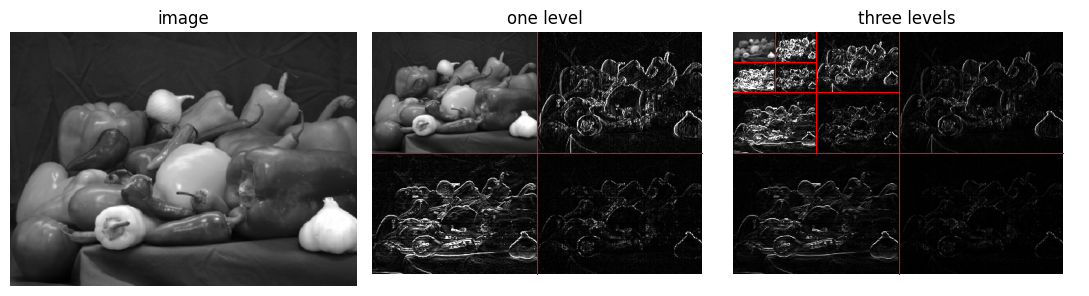

haar_step_2d reuses the 1D step: once along the rows (the last axis), then, after transposing so that the columns are along the last axis, once down the columns. haar_2d repeats the step on the top-left quadrant only, since that’s the approximation. In the display, the approximation is shown as an ordinary image, and the details by their magnitude, so that black means a coefficient near zero.

After one level (middle), the top-left quadrant is a half-size copy of the peppers, and the other three quadrants are mostly black, bright only along edges: the top-right quadrant lights up on the near-vertical edges of the peppers, the bottom-left on the horizontal ones, and the bottom-right, diagonal detail, is the darkest. After three levels (right), the approximation is $1/8$ the size in each direction, and we have details at three scales, nested in the familiar pyramid layout.

Count the coefficients: the pyramid has exactly as many as the image has pixels. Nothing has been compressed yet. But the image’s energy has been rearranged so that it’s concentrated in a small corner, and most of the remaining coefficients are nearly zero.

C = haar_2d(I, 3)
energy = C**2
h, w = I.shape[0] >> 3, I.shape[1] >> 3
print(f'the approximation is {h * w / I.size:.1%} of the coefficients, '
      f'holding {energy[:h, :w].sum() / energy.sum():.2%} of the energy')
print(f'energy preserved: image {np.sum(I**2):.2f}, coefficients {energy.sum():.2f}')

the approximation is 1.6% of the coefficients, holding 97.74% of the energy
energy preserved: image 22050.54, coefficients 22050.54

The approximation, under 2% of the coefficients, holds nearly all of the energy. The second line checks that the total energy is unchanged, as it must be for an orthonormal transform: the Haar transform only redistributes the energy.

To undo the transform, we undo each step in reverse order, starting from the coarsest level. Each 1D step is undone with $p_0 = (c_0 + c_1)/\sqrt{2}$ and $p_1 = (c_0 - c_1)/\sqrt{2}$ .

def inverse_haar_step_1d(a, d):
    '''Undo haar_step_1d: interleave (a + d)/sqrt(2) and (a - d)/sqrt(2).'''
    x = np.empty(a.shape[:-1] + (2 * a.shape[-1],))
    x[..., 0::2] = (a + d) / np.sqrt(2)
    x[..., 1::2] = (a - d) / np.sqrt(2)
    return x

def inverse_haar_step_2d(C):
    h, w = C.shape
    T = C.T                                                    # undo the column step first...
    rows_done = inverse_haar_step_1d(T[:, :h // 2], T[:, h // 2:]).T
    return inverse_haar_step_1d(rows_done[:, :w // 2], rows_done[:, w // 2:])   # ...then the rows

def inverse_haar_2d(C, levels):
    R = C.copy()
    h, w = C.shape[0] >> (levels - 1), C.shape[1] >> (levels - 1)
    for _ in range(levels):                                    # coarsest level first
        R[:h, :w] = inverse_haar_step_2d(R[:h, :w])
        h, w = 2 * h, 2 * w
    return R

print('largest reconstruction error:', np.abs(inverse_haar_2d(haar_2d(I, 3), 3) - I).max())

largest reconstruction error: 1.4432899320127035e-15

Perfect reconstruction, up to floating-point round-off.

Compression: Keeping the Largest Coefficients¶

Here’s the payoff. Since most coefficients are tiny, let’s keep only the largest ones (in magnitude) anywhere in the pyramid, set all the rest to zero, and reconstruct. Storing a mostly-zero pyramid takes far fewer bits than storing every pixel. (A real codec would also need to record which coefficients it kept, and would entropy-code the values; we’ll ignore that here.)

To measure the loss we’ll use the peak signal-to-noise ratio, the standard measure of reconstruction quality:

\text{PSNR} = 10 \log_{10} \frac{\text{peak}^2}{\text{MSE}} \ \text{dB},

where the peak is 1 for our image in $[0, 1]$ and MSE is the mean squared error. Higher is better. As a rough guide, above about 40 dB the differences are essentially invisible, and below about 30 dB they’re easy to see.

LEVELS = 5

def keep_largest(C, fraction):
    '''Zero all but the given fraction of coefficients with the largest magnitude.'''
    cutoff = np.quantile(np.abs(C), 1 - fraction)
    return np.where(np.abs(C) >= cutoff, C, 0)

def psnr(I, J):
    return 10 * np.log10(1 / np.mean((I - J)**2))

C = haar_2d(I, LEVELS)
fractions = [0.20, 0.05, 0.01]

fig, ax = plt.subplots(1, 4, figsize=(12, 3), sharex=True, sharey=True)
ax[0].imshow(I, cmap='gray'); ax[0].set_title('original')
for a, f in zip(ax[1:], fractions):
    R = inverse_haar_2d(keep_largest(C, f), LEVELS)
    a.imshow(np.clip(R, 0, 1), cmap='gray')
    a.set_title(f'{f:.0%} kept: {psnr(I, R):.1f} dB')
for a in ax:
    a.set_axis_off()
plt.tight_layout()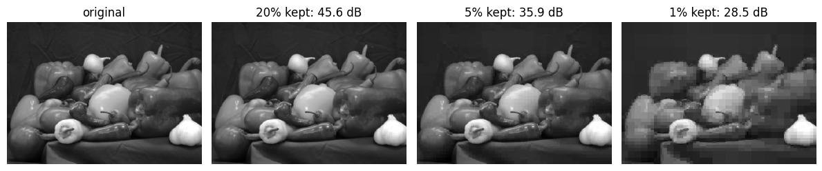

Keeping 20% of the coefficients, a 5-fold reduction in the numbers we store, the reconstruction is hard to tell from the original. At 5% it still looks good at a glance, though zooming in shows a slight blockiness in smooth regions. At 1% the blocks are obvious. Those blocks are the shapes of the Haar basis patterns themselves: every Haar pattern is piecewise constant, so with only a few of them we can only build piecewise-constant approximations. Even so, the garlic and the outlines of the peppers are still easy to make out with only 1 coefficient in 100, because the coefficients that sit on strong edges are exactly the large ones we kept.

Interactive Compression¶

Slide the fraction of coefficients kept, on a log scale from 0.1% to 100%.

pass  # (static) plt.ioff()
slider = FloatLogSlider(value=0.05, base=10, min=-3, max=0, step=0.1, description='kept')

fig, ax = plt.subplots(1, 2, figsize=(9, 3.5), sharex=True, sharey=True)
fig.canvas.header_visible = False
ax[0].imshow(I, cmap='gray', vmin=0, vmax=1)
R = inverse_haar_2d(keep_largest(C, slider.value), LEVELS)
rdisp = ax[1].imshow(np.clip(R, 0, 1), cmap='gray', vmin=0, vmax=1)
rtitle = ax[1].set_title(f'{slider.value:.1%} kept: {psnr(I, R):.1f} dB')
for a in ax:
    a.set_axis_off()

def update(change):
    R = inverse_haar_2d(keep_largest(C, slider.value), LEVELS)
    rdisp.set_data(np.clip(R, 0, 1))
    rtitle.set_text(f'{slider.value:.1%} kept: {psnr(I, R):.1f} dB')
    fig.canvas.draw()
    fig.canvas.flush_events()

slider.observe(update, names='value')

pass  # (static) VBox([slider, fig.canvas])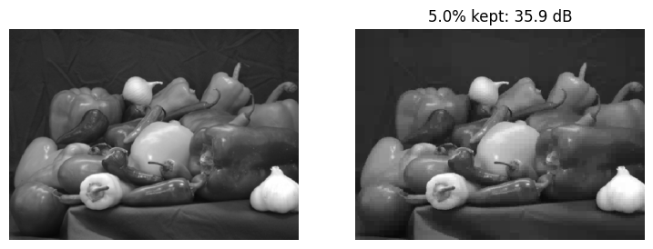

Wavelets and JPEG 2000¶

The original JPEG standard, which you’ll build parts of in the JPEG exercise, cuts the image into independent $8 \times 8$ blocks and transforms each with the DCT. Its successor, JPEG 2000, uses a wavelet pyramid over the whole image instead, like the one we built here. That brings several advantages:

No block boundaries. At high compression, JPEG’s independent blocks show visible seams between them. A whole-image wavelet transform has no fixed block grid.
Smoother wavelets. Our blockiness comes from the Haar patterns being piecewise constant. JPEG 2000 uses smoother wavelets (the CDF 9/7 and 5/3 wavelets), whose patterns overlap and taper, so heavy compression produces blur rather than blocks.
Multiple resolutions for free. The pyramid contains the image at every scale: the approximation at each level is a thumbnail. A JPEG 2000 file can be decoded at low resolution, or progressively refined as more data arrives, without storing separate versions.

Despite this, JPEG 2000 never displaced JPEG on the web: it’s more complex and slower to encode and decode, and JPEG was already everywhere. But it’s widely used in digital cinema, medical imaging, and archives. And the ideas, multi-scale decomposition and sparse coefficients, run through all of modern image processing.

🔨 Your Turn: Denoising by Shrinking Coefficients¶

Compression throws away small coefficients because they carry little of the image. But noise is spread evenly over all coefficients, so the small ones are mostly noise. That suggests using the same idea to remove noise.

Task: Add Gaussian noise (standard deviation 0.05) to the grayscale peppers image I. Remove as much of it as you can by shrinking the detail coefficients of its Haar pyramid toward zero, and reconstruct. Compare your result, in PSNR against the clean image and by eye, with simply blurring the noisy image using gaussian_filter at its best $\sigma$ .

Guidance:

Leave the approximation (the top-left corner of the pyramid) alone: it holds the image’s large-scale content, and only a little of the noise.
Two common rules: hard thresholding sets every detail coefficient with magnitude below a threshold $\lambda$ to zero and leaves the others alone; soft thresholding also shrinks the survivors toward zero by $\lambda$ . Try both. np.sign and np.maximum are useful for the second.
Because the transform is orthonormal, the noise in each coefficient has the same standard deviation as the noise in each pixel. Try thresholds that are a small multiple of that.
Compute the PSNR for a range of thresholds and plot it, rather than guessing one. Do the same for the blur’s $\sigma$ .
Where does each method do better: in smooth regions, or along edges?

🧠 Further Efforts¶

Blocks or pyramid? Show that three levels of our whole-image Haar transform produce exactly the same coefficients as transforming every $8 \times 8$ block with make_haar_matrix(8), as in basis_decomp_64pix, just arranged differently. Why must that be true?
Guidance: Think about the support of each Haar pattern. Which pixels can a coefficient at the third level depend on? Check numerically with a single block first: transform an $8 \times 8$ image both ways.
Color. Compress a color image by applying the pyramid to each channel. Then convert to YCbCr first, and keep a smaller fraction of coefficients in the two color channels than in the luminance. Which approach gives a better-looking result for the same total number of coefficients?
Guidance: Compare at a matched total number of kept coefficients, and convert back to RGB before measuring PSNR or displaying.
Smoother wavelets. The PyWavelets package (uv add pywavelets) implements many wavelets. Use pywt.wavedec2 and pywt.waverec2 with 'haar' to check against our version, and then with 'bior4.4' (essentially JPEG 2000’s CDF 9/7 wavelet). Keeping 1% of the coefficients, compare the artifacts.
Guidance: pywt.coeffs_to_array turns the list of subbands into a single array, so keep_largest works on it unchanged.