Viewing different basis blocks, along with their transform matrices

stough 202-

DIP Chapter 6, 8.9

Discrete wavelets broadly can be seen as a way of looking at a signal as a collection of patterns instead of as a collection of independent samples. In order to uniquely and fully describe a signal, these basis patterns should be orthogonal to one another (all dot products zero), have magnitude 1, and cover the space of all possible signals. For us, the signal is a NxN block of pixels within an image. wavelet_utils provides numerous orthonormal basis sets for the block size of our choosing. Here, we look at them in turn.

When I talk about the power of any basis, I am thinking of how efficient any such basis will be in terms of concentrating the signal in as few coefficients (basis patterns) as possible. This is also dependent on the kind of image data being considered.

Markdown latex equations

%matplotlib inline
import matplotlib.pyplot as plt
import numpy as np

# For importing from alternative directory sources
import sys  
sys.path.insert(0, '../dip_utils')

from matrix_utils import (arr_info,
                          make_linmap)
from vis_utils import (vis_image,
                       vis_rgb_cube,
                       vis_hists,
                       vis_pair,
                       vis_surface)

from wavelet_utils import (make_haar_matrix,
                           make_random_basis,
                           make_klt_basis,
                           make_dct_matrix,
                           make_standard_matrix,
                           vis_blocks)

First up, the standard, or Euclidean matrix.¶

This is the most natural basis, and the one you think about when you imagine a block to consist of a collection of pixels.

\mathbf{H_{Euc}} = \begin{vmatrix} 1 & 0 & 0 & 0\\ 0 & 1 & 0 & 0 \\ 0 & 0 & 1 & 0 \\ 0 & 0 & 0 & 1 \end{vmatrix}

If we consider just the 2D (2x2) version:

\mathbf{H_{Euc}} = \begin{vmatrix} 1 & 0 \\ 0 & 1 \end{vmatrix}

This is how you describe any location in a Cartesian 2D space. This is a basis pattern, where each coefficient will precisely reflect the signal in just one of the two pixels. Recall, these basis patterns should be orthogonal to one another, have magnitude 1, and cover the space of all possible signals. So

$\langle 1,0 \rangle \cdot \langle 0,1 \rangle = 0$ , so the basis is orthogonal
Each of $\langle 1,0 \rangle$ and $\langle 0,1 \rangle$ has magnitude 1 (square root of the sum of squares of the components).
We know every point in 2D can be described with a coordinate in x and a coordinate in y. Or, a coefficient with respect to $\langle 1,0 \rangle$ and a coefficient with respect to $\langle 0,1 \rangle$ .

We take outer products of the rows to extend this basis set to square-sized basis patterns.

Euc = make_standard_matrix(4)
vis_blocks(Euc)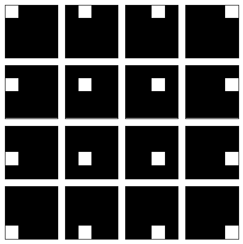

Next up, the Haar matrix.¶

Most useful basis sets will account for spatial coherence by incorporating the mean as one of the basis vectors. If there is just one piece of information you can store about a block, the mean intensity of the block would be the first choice. The Haar basis construction can be found analytically in DIP 6.9, with the implementation details available to you in waveletUtil.py.

\mathbf{H_{Haar}} = \frac{1}{2}\begin{vmatrix} 1 & 1 & 1 & 1\\ 1 & 1 & -1 & -1 \\ {\sqrt 2} & -{\sqrt 2} & 0 & 0 \\ 0 & 0 & {\sqrt 2} & -{\sqrt 2} \end{vmatrix}

If we consider just the 2D (2x2) version:

\mathbf{H_{Haar}} = \frac{1}{\sqrt 2}\begin{vmatrix} 1 & 1 \\ 1 & -1 \end{vmatrix}

Rather than store a coefficient for each pixel as the Euclidean basis does, this seems to dedicate one coefficient to the average of the two pixels and one coefficient to difference between the two. This is also a basis pattern. Recall, these basis patterns should be orthogonal to one another, have magnitude 1, and cover the space of all possible signals. So

$\langle \frac{1}{\sqrt 2}, \frac{1}{\sqrt 2} \rangle \cdot \langle \frac{1}{\sqrt 2},-\frac{1}{\sqrt 2} \rangle = 0$ , so the basis is orthogonal
E.g.: $\langle \frac{1}{\sqrt 2}, -\frac{1}{\sqrt 2} \rangle$ has magnitude 1: $\Bigl( \frac{1}{\sqrt 2} \Bigr)^2 + \Bigl( -\frac{1}{\sqrt 2} \Bigr)^2 = 1$
The basis covers all possible signals, here points in 2D:

\forall (x,y) \in R^2, \verb+let+ \\ a = \langle \frac{1}{\sqrt 2}, \frac{1}{\sqrt 2} \rangle \cdot \langle x,y \rangle = \frac{x + y}{\sqrt 2}\\ b = \langle \frac{1}{\sqrt 2}, -\frac{1}{\sqrt 2} \rangle \cdot \langle x,y \rangle = \frac{x - y}{\sqrt 2}.\\ \verb+Then+ \\ a\langle \frac{1}{\sqrt 2}, \frac{1}{\sqrt 2} \rangle + b\langle \frac{1}{\sqrt 2}, -\frac{1}{\sqrt 2} \rangle \\ = \Bigl( \frac{x + y}{\sqrt 2} \Bigr)\langle \frac{1}{\sqrt 2}, \frac{1}{\sqrt 2} \rangle + \Bigl( \frac{x - y}{\sqrt 2} \Bigr)\langle \frac{1}{\sqrt 2}, -\frac{1}{\sqrt 2} \rangle \\ = \langle \frac{x + y}{2}, \frac{x + y}{2} \rangle + \langle \frac{x - y}{2}, \frac{-x + y}{2} \rangle \\ = \langle \frac{2x + y - y}{2}, \frac{x - x + 2y}{2} \rangle \\ = \langle x,y \rangle

Haar = make_haar_matrix(4)
vis_blocks(Haar)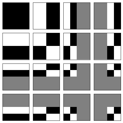

Next up, the Discrete Cosine transform matrix.¶

Each row of this matrix represents a sampled cosine wave with varying frequency over the signal space (s-D space, where s is the number of pixels). In that it satisfies the three conditions we specified above (left to you to prove), it can serve just as well as either of the above two. It is based in Fourier analysis on the idea that any signal can be constructed from cosine and sine waveforms.

The DCT is even more powerful for natural images because unlike the above two, here every basis pattern extends over the whole block. In fact, some form of DCT is usually so powerful, it has been adopted for use in JPEG, MPEG, and many other image and video compression standards.

Recall $s$ is the number of pixels, i.e. the size of our square matrix. The first row is again the mean, while later rows ( $u$ ) are sampled (by column $j$ ) cosines:

DCT_0 = \sqrt \frac{1}{s} \\ DCT_u = \sqrt \frac{2}{s}cos\Bigl(\frac{(2j+1)u\pi}{2s}\Bigr), j = 0,\dots,s-1, u = 1,\dots,s-1

DCT = make_dct_matrix(4)
print(DCT)

[[ 0.5         0.5         0.5         0.5       ]
 [ 0.65328148  0.27059805 -0.27059805 -0.65328148]
 [ 0.5        -0.5        -0.5         0.5       ]
 [ 0.27059805 -0.65328148  0.65328148 -0.27059805]]

vis_blocks(DCT)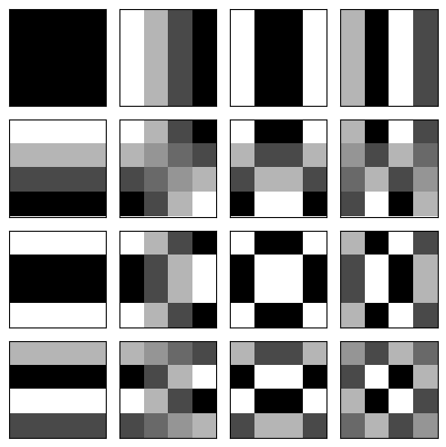

# View some of these supposedly orthogonal vectors... 
DCT16 = make_dct_matrix(16)
plt.figure()
plt.plot(DCT16[:4,:].T)
plt.legend(['row 0', 'row 1', 'row 2', 'row 3', 'row 4']);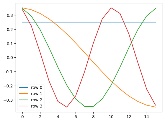

np.dot(DCT16[10,:], DCT16[5,:])

np.float64(1.1102230246251565e-16)

np.sum(DCT16[3,:]**2)

np.float64(0.9999999999999999)

# A more detailed view of these basis patterns as height maps.
DCT128 = make_dct_matrix(128) # So large just for visualization.
vis_surface(np.outer(DCT128[2,:], DCT128[4,:]))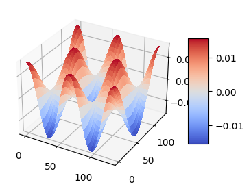

Random: with the magic of Gram-Schmidt¶

orthonormalization, we can actually make a basis from any set of N vectors in N-D, as long as no one of them can be written as a linear combination of the others. There is of course no telling how powerful any such basis will be in terms of concentrating the signal in as few coefficients (basis patterns) as possible.

Hrnd = make_random_basis(4)
vis_blocks(Hrnd)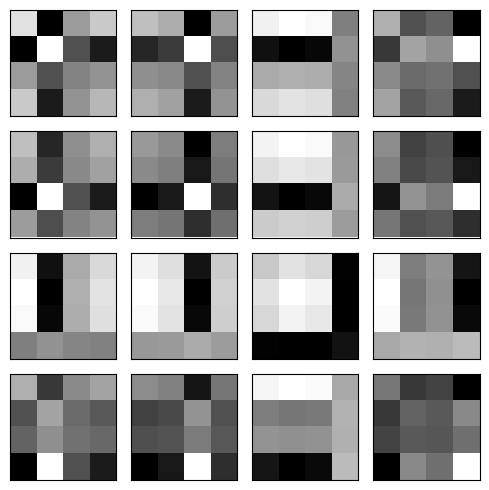

Principal Component Analysis (PCA):¶

Rather than either a predefined basis (e.g., Euclidean, Haar, DCT) or a random basis, let’s make a basis that is ideal for the data that we want to compress.

Principal components analysis is a much larger topic than we can cover just yet here, but if you’re interested, take a look at this youtube channel. For us, PCA finds directions in the data space that account for the most variance in the data. That is, the first basis pattern PCA will compute is the one that accounts for as much of all the data differences as possible. After that, PCA will compute an orthogonal direction that accounts for as much of what’s left as possible.

Here, and unlike the previous cases, we need the image data that we’re interested in.
Unlike the predefined cases, we would have to explicitly send the transform matrix along with the coefficients to allow the receiving end to decode. This is like Huffman coding, where we construct just the right encoder/decoder to do the best job on the data at hand.
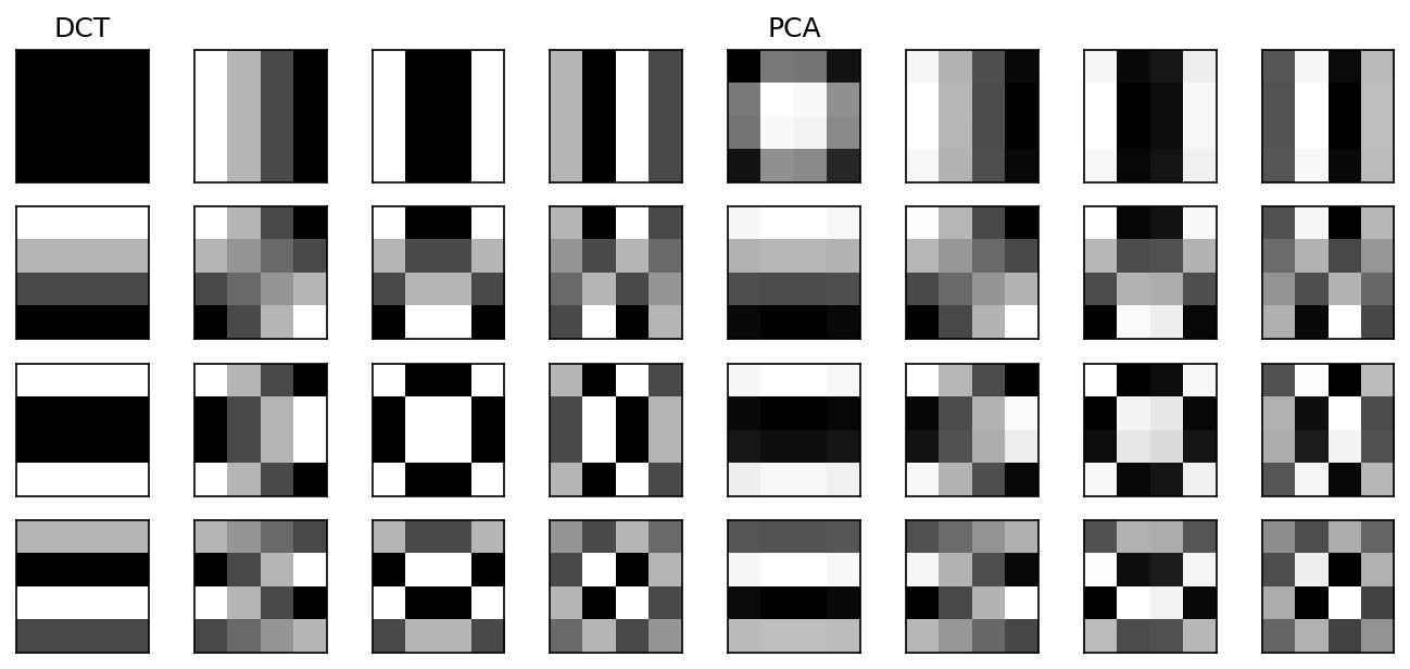
Using a pretty small size (like 4), PCA on many natural images will lead to a basis that bears some resemblance to DCT. This is congruent with what we have been told about the power of the DCT transform: on lots of natural images, the DCT is close to as good as it gets (which is PCA).

I = plt.imread('../dip_pics/happy128.png').astype(np.float32)
vis_image(I)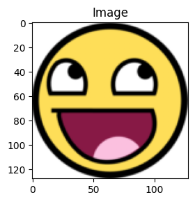

Hpca = make_klt_basis(I, size=4)
vis_blocks(Hpca)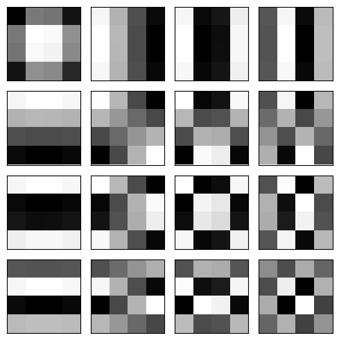

# Notice that the PCA ends up looking like a lot like the DCT. 
# That says something about the predefined DCT on natural images. 
f, ax = plt.subplots(4,8, figsize=(9,4))
vis_blocks(DCT, ax[:,:4])
vis_blocks(Hpca, ax[:,4:])
ax[0][0].set_title('DCT');
ax[0][4].set_title('PCA');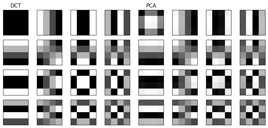

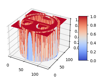
vis_surface(I[...,0])