Spatial Coherence and Change of Basis - imageprocessing-awesome

Preview: Spatial Coherence and Change of Basis

stough, 202-

Khan Academy on Change of Basis

Complicated way of saying it: Image compression relies on spatial coherence of image data. The fact that a pixel’s value is highly correlated with its neighbors most of the time, means that changes of basis like the below can lead to a much more compressible coordinate representation (more zeros, or minimum description length)...

Little simpler: We are all familiar with plotting points in the plane.

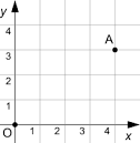
A point $A$ for example might have the coordinates $\langle4,3\rangle$ , by which we mean $4\cdot\langle1,0\rangle + 3\cdot\langle0,1\rangle$ , or 4 in the $x$ direction and 3 in the $y$ . But the same point in space can also be represented as for example $3.5\cdot\langle1,1\rangle + 0.5\cdot\langle1,-1\rangle$ , or rather $\langle\frac{7}{\sqrt2}, \frac{1}{\sqrt2}\rangle$ if we insist on the two directions we’re measuring in ( $\langle1,1\rangle,\langle1,-1\rangle$ ) to be unit length.

If we think about the magnitude or energy of the point, or distance from the origin, notice that in this alternative representation, much of that magnitude ( $\frac{7}{8}$ th of it in fact) is accounted for by the first component. In fact for a lot of points for which the $x$ and $y$ components are nearly the same, the second component could potentially be ignored without losing too much. This is where the compression will come from: if we can ignore the coefficient with some minimal loss, then we don’t have to store or transmit it.

In this demo we’re going to try to demonstrate how such a change of basis can improve the compressibility of image data. We’ll look at a pixel and its neighbor, over all pairs in an image. Spatial coherence implies that most of the time, a pixel and its neighbor will be similar.

%matplotlib inline
import matplotlib.pyplot as plt
import numpy as np

# For importing from alternative directory sources
import sys  
sys.path.insert(0, '../dip_utils')

from matrix_utils import (arr_info,
                          make_linmap)

from vis_utils import (vis_image,
                       vis_pair,
                       vis_triple)

I = plt.imread('../dip_pics/cat_small.png')
arr_info(I)

((512, 512, 4), dtype('float32'), np.float32(0.0), np.float32(1.0))

vis_image(I, show_ticks=False, title=None)

vis_image(I[...,0], show_ticks=False, title=None, cmap='gray', interpolation=None)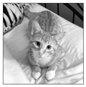

Let’s look at pixel pairs¶

We’ll just consider one of the color channels so as not to confuse the issue more.

pix_pairs = np.reshape(I[...,0], (-1,2)).copy()
arr_info(pix_pairs)

((131072, 2), dtype('float32'), np.float32(0.0), np.float32(0.9882353))

pix_pairs[:10]

array([[0.76862746, 0.78039217],
       [0.78039217, 0.7764706 ],
       [0.7764706 , 0.78431374],
       [0.78431374, 0.78039217],
       [0.78431374, 0.76862746],
       [0.67058825, 0.49803922],
       [0.27058825, 0.14901961],
       [0.14117648, 0.14117648],
       [0.15294118, 0.14509805],
       [0.14509805, 0.15686275]], dtype=float32)

numpoints = 5000
randomInds = np.random.choice(pix_pairs.shape[0], numpoints, replace=False)

f, ax = plt.subplots()
ax.scatter(pix_pairs[randomInds,0], pix_pairs[randomInds,1], alpha=.05)
ax.set_aspect('equal')
ax.set_xlabel(r'$pix_i$')
ax.set_ylabel(r'$pix_{i+1}$')
ax.set_title('Pixel pair scatter');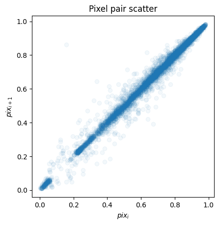

It looks like neighboring pixels are highly correlated with one another. This is the essence of spatial coherence. Rather than considering them as independent pieces of information, we can instead reframe how we represent a pixel pair.

Changing the basis of a pixel pair¶

If we want to reframe every pixel pair to take advantage of spatial coherence, we can move from the independent basis $\{\langle1,0\rangle,\langle0,1\rangle\}$ to a different independent basis like $\{\frac{1}{\sqrt2}\langle1,1\rangle,\frac{1}{\sqrt2}\langle1,-1\rangle\}$ . Rather than thinking of the pixel pair as “this pixel, then that pixel”, we’ll have something like “the average of the pair, then the difference of the pair.” If spatial coherence is as prevelent as the above scatter plot implies, then “the difference of the pair” will be a relatively insignificant part of the typical pair.

To transform the normal representation of a pixel pair $\langle pix_0,pix_1\rangle$ to the new basis, we can multiply it by a matrix of the two new basis vectors:

\frac{1}{\sqrt2}\begin{vmatrix} 1 & 1 \\ 1 & -1 \end{vmatrix} \begin{vmatrix} pix_0 \\ pix_1 \end{vmatrix} = \frac{1}{\sqrt2}\begin{vmatrix} pix_0 + pix_1 \\ pix_0 - pix_1 \end{vmatrix} = \begin{vmatrix} c_0 \\ c_1 \end{vmatrix}

You can check this with respect to the pixel pair $\langle4,3\rangle$ noted at the top. Below we’ll call this representation avg/diff. (It’s also the first steps to the Haar wavelet basis.)

H = np.array([[1, 1],[1, -1]])/np.sqrt(2)

array([[ 0.70710678,  0.70710678],
       [ 0.70710678, -0.70710678]])

# H is 2x2, while the pix_pairs is Nx2.  So
# we transpose the pix_pair to get 2xN. The
# result of the matmul is 2xN, then we transpose it back.
new_coords = np.matmul(H, pix_pairs.T).T
arr_info(new_coords)

((131072, 2),
 dtype('float64'),
 np.float64(-0.49913420034404155),
 np.float64(1.3948027891445542))

np.mean(new_coords, axis=0)

array([ 9.02026491e-01, -1.25878487e-05])

When we compute the average coefficient in the avg versus the diff dimensions, we can see that on average, the first coefficient has much more power. Again, this is expected given that we saw above how correlated neighboring pixel values are.

Let’s see how much energy is in each component for each pair.¶

We would like to understand what percentage of the total is in each component in this new representation. We want each pair to sum to 1, where the components are positive.

# We want to use the absolute values, and divide by the sum so that the sum of each pair is one.
# The np.abs(new_coords) will have shape (N,2), whereas the .sum(axis=-1) produces a (N,). 
# In order to broadcast the shapes correctly, we can add [:,None] so that we're dividing 
# (N,2) with (N,1), and numpy will know what that means. Or just keepdims!
normed_coords = np.abs(new_coords) / np.abs(new_coords).sum(axis=-1, keepdims=True)

normed_coords[:10]

array([[9.92462312e-01, 7.53768787e-03],
       [9.97487437e-01, 2.51256262e-03],
       [9.95000000e-01, 4.99999962e-03],
       [9.97500000e-01, 2.49999981e-03],
       [9.90000001e-01, 9.99999924e-03],
       [8.71345018e-01, 1.28654982e-01],
       [7.75362316e-01, 2.24637684e-01],
       [1.00000000e+00, 6.72321969e-18],
       [9.74358977e-01, 2.56410231e-02],
       [9.62500004e-01, 3.74999964e-02]])

normed_coords[:10].sum(axis=-1, keepdims=True)

array([[1.],
       [1.],
       [1.],
       [1.],
       [1.],
       [1.],
       [1.],
       [1.],
       [1.],
       [1.]])

You can see that, at least for the first ten pixel pairs, that in this new representation the energy in the $\frac{1}{\sqrt2}\langle1,1\rangle$ direction is most of the total. Let’s look at a histogram of these two components, to see if this trend holds across the whole image.

bins = np.arange(0,1, 1/400)

f, ax = plt.subplots()
ax.hist(normed_coords[:,0], bins, alpha = .6, label = r'$c_0$', color = 'r');
ax.hist(normed_coords[:,1], bins, alpha = .6, label = r'$c_1$', color = 'b');

plt.legend();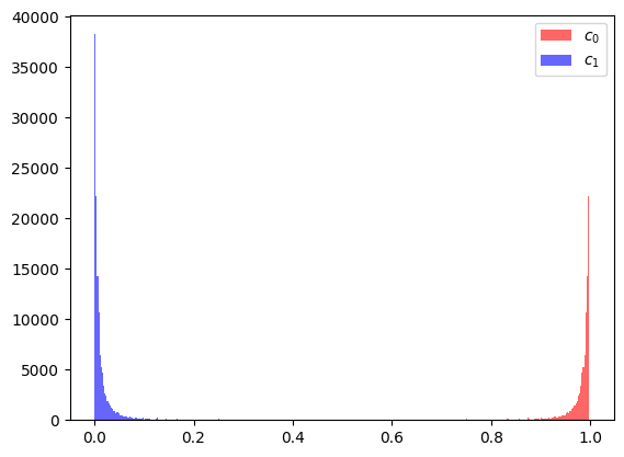

It looks like in the new representation, the $c_0$ component, associated with the $\frac{1}{\sqrt2}\langle1,1\rangle$ direction, has almost all the power/energy/magnitude associated with any pair. How does this compare to the original representation?

normed_pix = np.abs(pix_pairs) / np.abs(pix_pairs).sum(axis=-1, keepdims=True)
bins = np.arange(normed_pix.min(), normed_pix.max(), 1/400)

f, ax = plt.subplots()
ax.hist(normed_pix[:,0], bins, alpha = .6, label = r'$pix_0$', color = 'r');
ax.hist(normed_pix[:,1], bins, alpha = .6, label = r'$pix_1$', color = 'b');

plt.legend();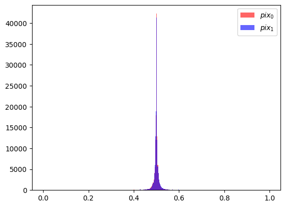

The above plot shows that when we consider a pair as two indpendent pixels, then each component ( $pix_i$ , and $pix_{i+1}$ ) is equally important.

What if we zeroed out all of that less important dimension?¶

Given that the $c_1$ components seem to matter so little, what if we just didn’t keep them? Would that change the image all that much? Once we’ve zeroed out the $c_1$ components, then going back to the pixel space is a matter of multiplying in the other direction:

\begin{vmatrix} c_0 & c_1 \end{vmatrix} \cdot \frac{1}{\sqrt2}\begin{vmatrix} 1 & 1 \\ 1 & -1 \end{vmatrix} = \frac{1}{\sqrt2}\begin{vmatrix} pix_0 + pix_1 & pix_0 - pix_1 \end{vmatrix} \cdot \frac{1}{\sqrt2}\begin{vmatrix} 1 & 1 \\ 1 & -1 \end{vmatrix} = \frac{1}{2}\begin{vmatrix} 2pix_0 & 2pix_1 \end{vmatrix} = \begin{vmatrix} pix_0 & pix_1 \end{vmatrix}

You can check with respect to the coefficient representation $\langle\frac{7}{\sqrt2}, \frac{1}{\sqrt2}\rangle$ from above.

new_coords[:,1] = 0

rec_pairs = np.matmul(new_coords, H.T)
arr_info(rec_pairs)

((131072, 2),
 dtype('float64'),
 np.float64(0.003921568859368562),
 np.float64(0.9862745106220244))

Ir = np.reshape(rec_pairs, I.shape[:2])

vis_pair(I[...,0], Ir, cmap='gray', show_ticks=False, second_title='Using only avg in avg/diff', interpolation=None)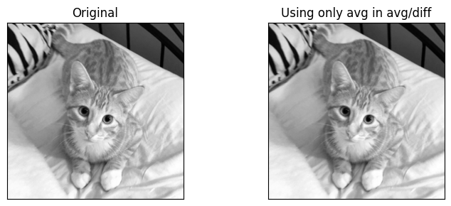

It appears that eliminating half of the coefficients (all of the $c_1$ ’s) has a neglible effect on the image. So, 50% compression with negligible fidelity loss.

How does this compare to eliminating one of the pixels in every pixel pair in the original representations?

pix_pairs[:,1] = 0 # also, could try pix_pairs[:,0]
Irp = np.reshape(pix_pairs, I.shape[:2])

vis_triple(I[...,0], Irp, Ir, cmap='gray', show_ticks=False, 
           second_title='Using half in pixel space', 
           third_title='Using half in avg/diff', interpolation=None)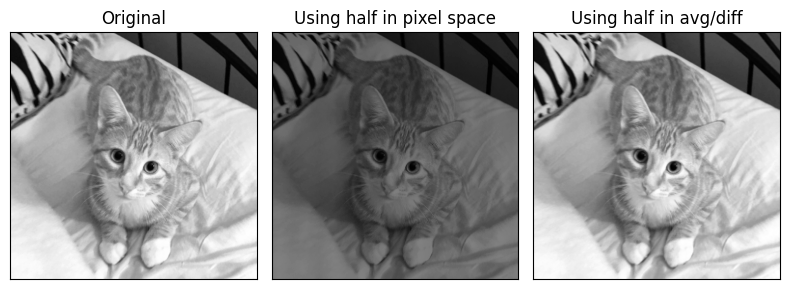

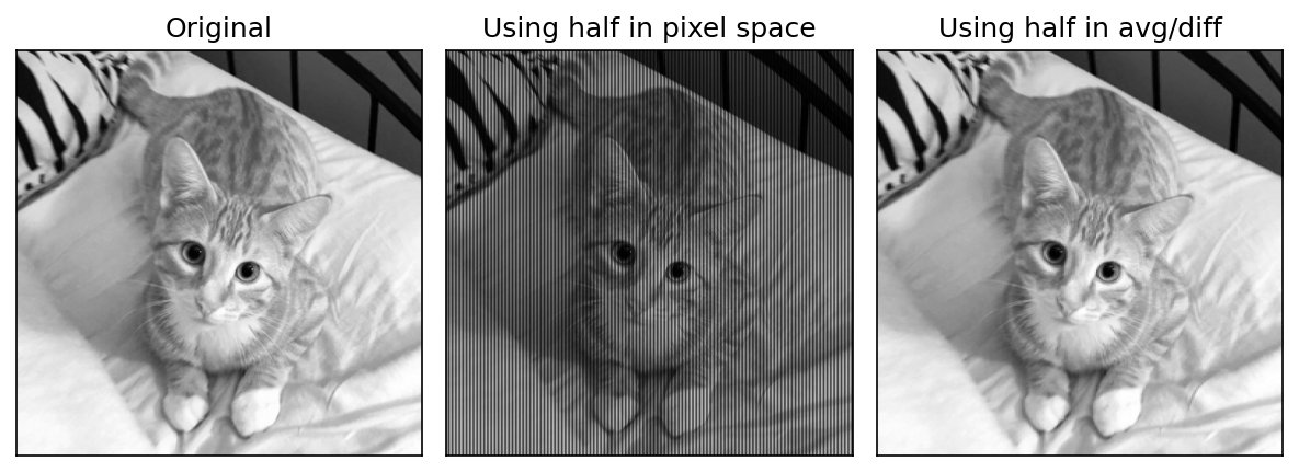
In the above we see that eliminating half of the coefficients in the pixel space leads to more noticeable degradation than doing so in the avg/diff representation. Due to spatial coherence, the avg/diff space usually accounts for most of the energy of a pixel pair in only the “avg” component. Such a change of basis followed by truncating or zeroing out components is the basis for lossy compression schemes like JPEG.

Little experiment figuring out how to consider a pixel and its horizontal neighbor.¶

a = np.arange(16).reshape(4,4)

array([[ 0,  1,  2,  3],
       [ 4,  5,  6,  7],
       [ 8,  9, 10, 11],
       [12, 13, 14, 15]])

np.reshape(a, (8,2))

array([[ 0,  1],
       [ 2,  3],
       [ 4,  5],
       [ 6,  7],
       [ 8,  9],
       [10, 11],
       [12, 13],
       [14, 15]])

np.reshape(a, (8,-1))

array([[ 0,  1],
       [ 2,  3],
       [ 4,  5],
       [ 6,  7],
       [ 8,  9],
       [10, 11],
       [12, 13],
       [14, 15]])

np.reshape(a, (-1,2))

array([[ 0,  1],
       [ 2,  3],
       [ 4,  5],
       [ 6,  7],
       [ 8,  9],
       [10, 11],
       [12, 13],
       [14, 15]])

Looking Ahead: the 2D Haar Transform on Image Blocks¶

We’ll see more on this later, but it’s worth mentioning now.

The 1D average/difference decomposition we’ve explored is the foundation of the 2D Haar wavelet transform. Here’s how it extends to 2D. Instead of a horizontal pair of pixels, take a $2 \times 2$ block

\begin{bmatrix} p_{00} & p_{01} \\ p_{10} & p_{11} \end{bmatrix}

and apply the same average/difference transform $H$ to its rows (the horizontal direction), and then to the columns of the result (the vertical direction). This produces four coefficients, each capturing a different kind of information:

LL (average in both directions): the block’s overall brightness. Taken over the whole image, the LL coefficients form a half-resolution copy of it.
LH (average along the rows, difference down the columns): responds where the intensity changes from top to bottom, that is, at horizontal edges.
HL (difference along the rows, average down the columns): responds to vertical edges.
HH (difference in both directions): diagonal detail and fine texture.

(Texts differ on which of the two mixed coefficients they call LH and which HL.) Because of spatial coherence, most of the image’s energy concentrates in the LL coefficients, while the other three are mostly near zero, so they can be coarsely quantized or discarded with little visible loss. Repeating the process on the LL image gives a multi-level decomposition. That is the idea behind wavelet compression schemes such as JPEG 2000. (The original JPEG uses a different transform, the discrete cosine transform, on $8 \times 8$ blocks.) We work through all of this in Haar Wavelets.