Glyph Image Converter - imageprocessing-awesome

A Block Transform Demo¶

stough 202-

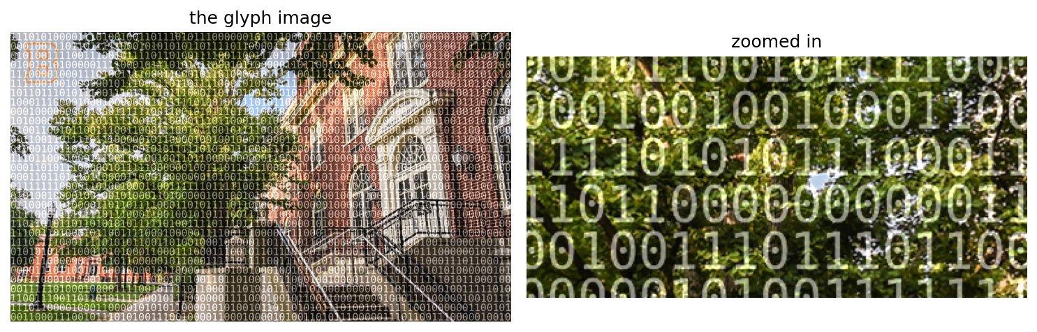
We saw in spatial filtering that a mask of weights is placed over each pixel in the image, followed by computing the inner product (sum of products) of the corresponding mask weights and pixel values. This resulted in a filtered image that might show a blurred version of the original, or else horizontal or vertical edges, or edginess generally, or any of a number of local spatial characteristics. But the spatial neighborhood represented by the mask moves by one pixel each iteration.

However, another way of viewing an image is as a grid of non-overlapping blocks, each block containing a number of pixels. A block transform is where we replace each block from the original image with a block of our choosing. We could choose to replace the whole collection of pixels in a block with the average or median color of the block. Or, as seen in this example, we can replace the block with a combination of the original block and a glyph image (basically, just a small image) that we’d like to overlay on our original.

Imports¶

We add several functions from the skimage module:

view_as_blocks decomposes an image into blocks of a defined size.
montage allows us to reassemble a bunch of blocks back into a grid.
We use resize or rescale to ensure that our image and glyphs have a common denominator that we can use as a block size.

%matplotlib inline
import matplotlib.pyplot as plt
import numpy as np

import skimage.color as color

# For importing from alternative directory sources
import sys  
sys.path.insert(0, '../dip_utils')

from matrix_utils import (arr_info,
                          make_linmap)
from vis_utils import (vis_rgb_cube,
                       vis_hists,
                       vis_pair)

from skimage.util import view_as_blocks
from skimage.util import montage
from skimage.transform import resize, rescale

I = plt.imread('../dip_pics/bucknellzoomb003.jpg')
vis_hists(I)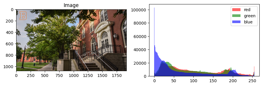

def get_glyphs(gsize=None):
    glyphs = np.stack([plt.imread(x) for x in [f'../dip_pics/{x:02b}.png' for x in range(4)]])
    
    if gsize is not None:
        if type(gsize)==list: 
            glyphs = np.stack([resize(glyph, gsize, order=0) for glyph in glyphs])
        else:
            glyphs = np.stack([rescale(glyph, gsize, order=0, channel_axis=-1) for glyph in glyphs])
    
    glyphs = (glyphs - glyphs.min())/(glyphs.max() - glyphs.min())
    
    return glyphs

glyphs = get_glyphs(.5)
print(arr_info(glyphs))

((4, 36, 47, 3), dtype('float32'), np.float32(0.0), np.float32(1.0))

plt.figure(figsize=(4,4))
plt.imshow(montage(glyphs, channel_axis=-1))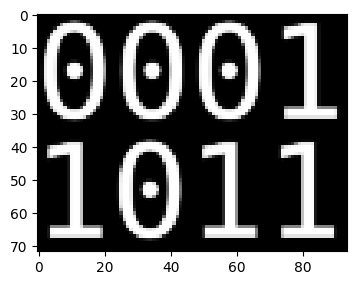

Our four glyphs are little images of the two-bit strings 00, 01, 10 and 11: white digits on black, here scaled to $36 \times 47$ pixels each. Every glyph has the same shape, which will be our block size.

[d+d%s for d,s in zip(I.shape[:2], glyphs.shape[1:3])]

[1080, 1960]

Ir = resize(I, [d+(s-d%s) for d,s in zip(I.shape[:2], glyphs.shape[1:3])])
vis_pair(I, Ir)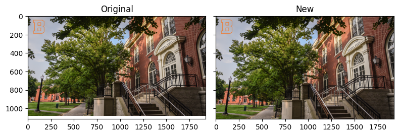

view_as_blocks needs the image dimensions to be exact multiples of the block size, so we resize the image up to the next multiple of the glyph size in each dimension. (The list comprehension in the cell before computes that new size: for each dimension d and block size s, d + (s - d % s).) The change is a few pixels at most, so the two look identical.

# size of blocks
block_shape = glyphs.shape[1:]

Ir = resize(I, [d+(s-d%s) for d,s in zip(I.shape[:2], glyphs.shape[1:3])])

# see the image as a matrix of blocks (of shape block_shape)
# Also, apply the JPEG -128 here.
view = view_as_blocks(Ir, block_shape)
view = np.squeeze(view)

view.shape

(31, 41, 36, 47, 3)

view is a 5D view into the image: a $31 \times 41$ grid of blocks, each block $36 \times 47 \times 3$ . It’s a view in the numpy sense: no pixels are copied, we’re just indexing the same memory differently. Reshaping to block_view flattens the grid into a single list of $31 \cdot 41 = 1271$ blocks that we can loop over.

block_view = view.reshape([view.shape[0]*view.shape[1]] + list(view.shape[2:]))

The block transform¶

Here’s where we decide what to do with each block. For every block we pick one of the four glyphs at random, and then combine the glyph with the block. The commented-out lines are alternatives I’ve played with, such as filling the glyph’s background with the block’s mean color, or coloring its digits with the complementary color. The active version is the last line: add half the glyph’s intensity on top of the block’s original pixels and clip, so the digits appear as a bright overlay. Try commenting it out and uncommenting one of the others.

#Compute all the transform coefficients.
#List of block transforms
glyph_view = np.zeros(block_view.shape)
rands = np.random.choice(len(glyphs), len(block_view))

for i in range(len(block_view)):
    block = block_view[i]
    block_mean = block.mean(axis=(0,1))
    
    color_glyph = glyphs[rands[i]].copy()
    
    mask = color_glyph[...,0] < .5
# #     mask = (grid_img>.5).sum()/grid_img.numel()
    
    # make background of the bit-glyph equal mean color of the block
#     color_glyph[mask] = block_mean

    # Make background of the bit-glyph exactly the block
#     color_glyph[mask] = block[mask]

    # Make the bit-glyph foregound just pop wrt to the block colors
#     color_glyph[mask] = block[mask]
#     color_glyph[~mask] = 1-block_mean
#     color_glyph[~mask] = 1-block[~mask]

    # Just an image of block means
#     color_glyph = block_mean
    
    # How about the bit-glyph background is the mean, foreground is complement.
#     color_glyph[mask] = block_mean
#     color_glyph[~mask] = 1-block[~mask]


    # How about some crazy alternative colorspace stuff?
    # Let's keep the background exactly the same. foreground is the opposite hsv
#     color_glyph[mask] = block[mask]
    
#     hsv = color.rgb2hsv(block_mean)
# #     hsv[0] = np.fmod(hsv[0]+.5, 1.0)
#     hsv[1:] = 1-hsv[1:]
#     block_mean_opp = color.hsv2rgb(hsv)
#     color_glyph[~mask] = block_mean_opp


    # How about ycbcr????
#     color_glyph[mask] = block[mask]
#     ybr = color.rgb2ycbcr(block_mean)
#     ybr[0] = 250.0-ybr[0]
    
#     block_mean_opp = color.ycbcr2rgb(ybr)
#     color_glyph[~mask] = block_mean_opp

    # This is just adding a fraction of the bit-glyph to the color.
    color_glyph = block + .5*color_glyph
    color_glyph = np.clip(color_glyph,0,1)
    
    

    glyph_view[i] = color_glyph

plt.figure(figsize=(8,5))
plt.imshow(montage(glyph_view, grid_shape=(view.shape[0], view.shape[1]), channel_axis=-1))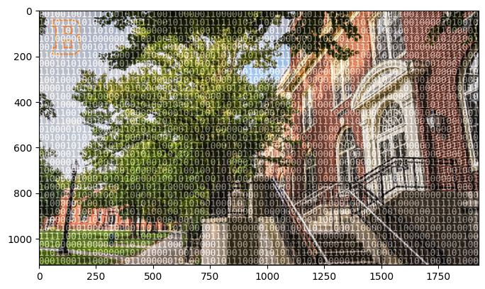

montage reassembles the list of processed blocks into the original grid layout. The result is our photo seemingly rendered in binary.

This is a playful example, but the structure (split into blocks, transform each block independently, reassemble) is exactly the structure of JPEG compression. There, the “transform” re-expresses each $8 \times 8$ block in terms of a set of basis patterns and throws away the patterns that matter least. Working block by block keeps the computation local and simple, at the cost of possible visible seams between blocks when the transform is too aggressive.

J = montage(glyph_view, grid_shape=(view.shape[0], view.shape[1]), channel_axis=-1)
plt.imsave('../dip_outs/binaryDana.png', J)