Otsu’s Method - imageprocessing-awesome

Thresholding from the Histogram¶

DRAFT, not finalized. This chapter is new and still under review.

stough 202-

Thresholding
Choosing a threshold: Otsu’s method
Implementing it
Interactive thresholding
Where one threshold fails
Local thresholds
🔨 Your Turn: Count the Coins
🧠 Further Efforts

Segmentation is the task of dividing an image into meaningful regions: the object and the background, the cells in a micrograph, the text on a page. It’s the step between processing an image and understanding it, since we can only measure, count, or recognize the things we’ve separated from their surroundings.

The simplest segmentation is thresholding: every pixel brighter than some value $t$ is foreground, and everything else is background. The whole difficulty is in choosing $t$ . In this notebook we’ll derive and implement the classic automatic choice, Otsu’s method (1979), which picks $t$ from nothing but the image’s histogram. Then we’ll see where any single threshold breaks down, and what to do about it.

%matplotlib inline
import matplotlib.pyplot as plt
import numpy as np
from skimage import data
from skimage.filters import threshold_otsu, threshold_local
from ipywidgets import VBox, IntSlider

# For importing from alternative directory sources
import sys
sys.path.insert(0, '../dip_utils')

from matrix_utils import arr_info
from vis_utils import vis_pair, vis_triple

Thresholding¶

Our test image is scikit-image’s coins, a photo of 24 old coins on a darker background, as 8-bit grayscale.

I = data.coins()
arr_info(I)

bins = np.arange(257)
hist, _ = np.histogram(I.ravel(), bins=bins)

fig, ax = plt.subplots(1, 2, figsize=(9, 3), gridspec_kw={'width_ratios': [1, 1.4]})
ax[0].imshow(I, cmap='gray')
ax[0].set_axis_off()
ax[1].bar(bins[:-1], hist, width=1)
ax[1].set_xlabel('intensity')
ax[1].set_ylabel('number of pixels')
plt.tight_layout()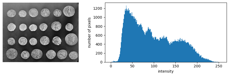

The histogram has a tall peak around 40 for the dark background, and a long, lumpy shoulder from about 80 to 200 for the coins, which are brighter and much more varied. It isn’t a textbook bimodal histogram, with two clean humps and an empty valley between them, but there’s clearly a dark population and a bright one, and a threshold somewhere between them should separate coins from background reasonably well. But where, exactly? We’d like a rule that picks the threshold automatically and reproducibly, without our eyeballing every image.

Choosing a Threshold: Otsu’s Method¶

Otsu’s idea: a good threshold splits the pixels into two classes that are each as uniform as possible. Think of it as the threshold that makes the two classes’ histograms as narrow as possible.

Let $p_k$ be the fraction of pixels with intensity $k$ (the histogram, normalized to sum to 1). A threshold $t$ splits the intensities into class 0, $k \le t$ , and class 1, $k > t$ . For each class we need its share of the pixels and its mean intensity:

\omega_0(t) = \sum_{k=0}^{t} p_k, \quad \omega_1(t) = 1 - \omega_0(t), \qquad \mu_0(t) = \frac{1}{\omega_0}\sum_{k=0}^{t} k\,p_k, \quad \mu_1(t) = \frac{1}{\omega_1}\sum_{k=t+1}^{255} k\,p_k.

“As uniform as possible” means a small within-class variance, $\sigma_W^2 = \omega_0\sigma_0^2 + \omega_1\sigma_1^2$ , the weighted average of the two classes’ variances. Here’s the key fact. The variance of all the pixels together, $\sigma_T^2$ , doesn’t depend on $t$ , and it splits into two parts:

\sigma_T^2 = \sigma_W^2(t) + \sigma_B^2(t), \qquad \text{where} \qquad \sigma_B^2(t) = \omega_0\,\omega_1\,(\mu_0 - \mu_1)^2

is the between-class variance: how far apart the two class means are, weighted by the class sizes. Since the total is fixed, minimizing the within-class variance is the same as maximizing the between-class variance. And $\sigma_B^2$ is much easier to compute, because it needs only the class sizes and means, not their variances.

So Otsu’s method is: compute $\sigma_B^2(t)$ for every possible threshold $t$ , and pick the $t$ where it’s largest. It rewards a split that is both balanced (the $\omega_0\omega_1$ factor is largest when the classes are of similar size) and well separated (the class means are far apart).

Implementing It¶

We could loop over the 256 thresholds, recomputing the sums each time. But every quantity above is a running sum over the histogram, which np.cumsum computes for every $t$ at once. With $m(t) = \sum_{k \le t} k\,p_k$ and the overall mean $\mu_T = m(255)$ , a little algebra (substitute $\mu_0 = m/\omega_0$ and $\mu_1 = (\mu_T - m)/\omega_1$ ) gives

\sigma_B^2(t) = \frac{\left(\mu_T\,\omega_0(t) - m(t)\right)^2}{\omega_0(t)\,\left(1 - \omega_0(t)\right)}.

def otsu(I):
    '''Return Otsu's threshold t for a uint8 image (foreground is I > t), and sigma_B^2 for every t.'''
    p = np.bincount(I.ravel(), minlength=256) / I.size   # normalized histogram
    k = np.arange(256)
    omega0 = np.cumsum(p)                                # class 0 share, for every t
    m = np.cumsum(k * p)                                 # running first moment
    muT = m[-1]                                          # overall mean
    with np.errstate(divide='ignore', invalid='ignore'):
        sigmaB2 = (muT * omega0 - m)**2 / (omega0 * (1 - omega0))
    sigmaB2 = np.nan_to_num(sigmaB2)                     # 0/0 where a class is empty
    return np.argmax(sigmaB2), sigmaB2

t, sigmaB2 = otsu(I)
print('our threshold:', t)
print('skimage threshold_otsu:', threshold_otsu(I))

our threshold: 107
skimage threshold_otsu: 107

The otsu function is a direct translation of the formula. np.bincount gives the histogram counts for each intensity 0 to 255, and dividing by the number of pixels makes it $p_k$ . The two cumsums compute $\omega_0(t)$ and $m(t)$ for all thresholds at once. At the extremes, one class is empty, the formula divides 0 by 0, and nan_to_num sets those to 0 so they can never win. np.argmax picks the best $t$ .

Our threshold agrees with scikit-image’s threshold_otsu, which uses the same convention: foreground is I > t. Let’s look at $\sigma_B^2(t)$ over the histogram, and at the segmentation.

fig, ax = plt.subplots(1, 2, figsize=(10, 3.2), gridspec_kw={'width_ratios': [1.4, 1]})
ax[0].bar(bins[:-1], hist, width=1, color='gray')
ax[0].set_xlabel('intensity')
ax[0].set_ylabel('number of pixels')
ax2 = ax[0].twinx()
ax2.plot(sigmaB2, 'C1', lw=2)
ax2.set_ylabel(r'$\sigma_B^2(t)$', color='C1')
ax[0].axvline(t, color='r', ls='--')
ax[0].set_title(f"Otsu's threshold t = {t}")

ax[1].imshow(I > t, cmap='gray')
ax[1].set_title('I > t')
ax[1].set_axis_off()
plt.tight_layout()

print(f'separability: sigma_B^2 / sigma_T^2 = {sigmaB2[t] / I.var():.2f}')

separability: sigma_B^2 / sigma_T^2 = 0.76

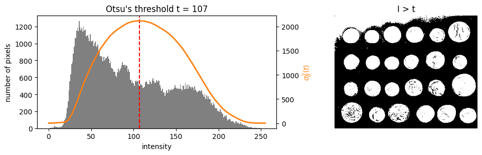
The orange curve, $\sigma_B^2(t)$ , rises smoothly to a single broad peak, between the background peak and the bulk of the coin pixels, and falls off toward the ends, where one class gets too small to matter. Its peak, the red dashed line, is Otsu’s threshold.

The printed separability, $\sigma_B^2 / \sigma_T^2$ , is the fraction of the image’s total variance that the two-class split explains. It’s between 0 and 1, and the closer to 1, the more cleanly the histogram splits into two. It’s a useful check on whether a two-class threshold even makes sense for an image.

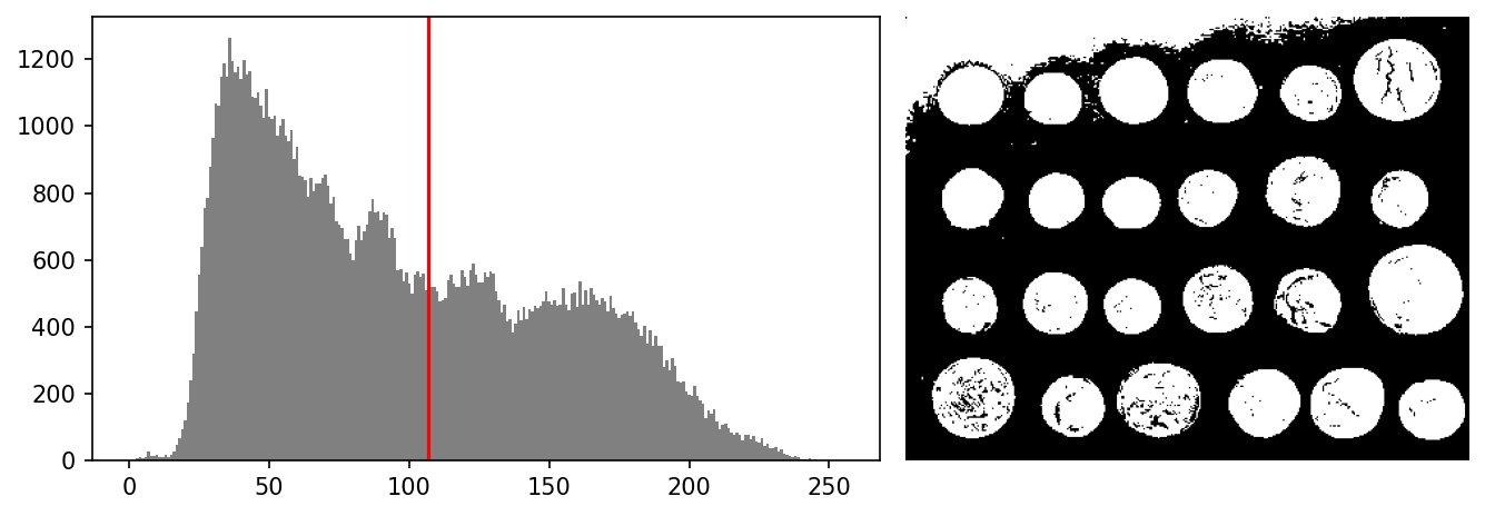
The segmentation is good but not perfect. Most coins come out as white disks, but several, especially in the bottom row, have dark speckles and cracks inside them where their own darker details fell below $t$ . And the background isn’t evenly lit: along the top edge, and especially at the top left, it’s brighter than elsewhere, and it comes out white, merging with the first coins. One global $t$ has to compromise between all parts of the image.

Interactive Thresholding¶

Drag the threshold to see how sensitive the result is. Start at Otsu’s $t$ and move a few steps either way.

pass  # (static) plt.ioff()
slider = IntSlider(value=int(t), min=0, max=255, description='threshold')

fig, ax = plt.subplots(1, 2, figsize=(9, 3.2), gridspec_kw={'width_ratios': [1.4, 1]})
fig.canvas.header_visible = False
ax[0].bar(bins[:-1], hist, width=1, color='gray')
line = ax[0].axvline(t, color='r')
bdisp = ax[1].imshow(I > t, cmap='gray')
ax[1].set_axis_off()
plt.tight_layout()

def update(change):
    line.set_xdata([slider.value, slider.value])
    bdisp.set_data(I > slider.value)
    fig.canvas.draw()
    fig.canvas.flush_events()

slider.observe(update, names='value')

pass  # (static) VBox([slider, fig.canvas])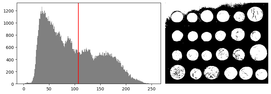

Where One Threshold Fails¶

Otsu’s method assumes that one threshold can separate foreground from background everywhere in the image. That assumption breaks when the lighting is uneven. Here’s scikit-image’s page sample, a photo of a printed page whose illumination falls off toward the left.

plt.ion()   # back to showing figures as they're made (the slider cell turned this off)

P = data.page()
arr_info(P)

tP, _ = otsu(P)
vis_pair(P, P > tP, cmap='gray', figsize=(10, 2.8), show_ticks=False,
         first_title='page', second_title=f'global Otsu, t = {tP}')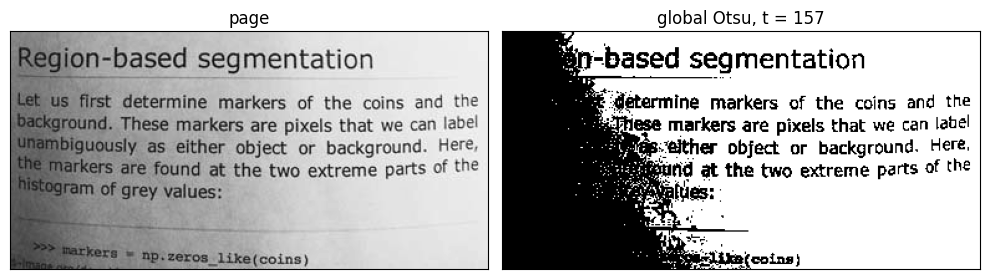

The global threshold does well where the paper is brightly lit, but toward the darker left side the paper itself falls below $t$ and turns black, swallowing the text. No single threshold can fix this: the paper at the far left (a median intensity of about 98) is darker than much of the ink on the right (whose darkest 5% are below about 105). You can check that with the interactive figure above, by setting I = P and re-running it.

Local Thresholds¶

The fix is to let the threshold vary across the image. A local (or adaptive) threshold computes a separate threshold for every pixel from its own neighborhood. Since what matters is whether a pixel is darker than its surroundings, a natural choice is the local mean, slightly offset:

t(i, j) = \bar{I}_{N(i,j)} - c

where $\bar{I}_{N(i,j)}$ is the mean over a window around pixel $(i, j)$ , which is exactly the low-pass filter we already know. threshold_local computes it (with a Gaussian-weighted mean by default), given an odd block_size for the window width and an offset $c$ .

T_local = threshold_local(P, block_size=35, offset=10)
arr_info(T_local)

vis_triple(P > tP, T_local, P > T_local, cmap='gray', figsize=(10, 2.8), show_ticks=False,
           first_title='global Otsu', second_title='local threshold t(i, j)', third_title='P > t(i, j)')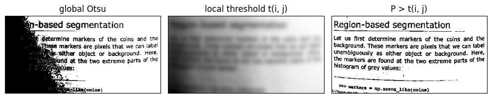

The middle panel is the threshold itself, an image: a smooth version of the page that is darker where the page is darker. Comparing each pixel against it (right) removes the effect of the lighting, and the text comes through cleanly across the whole page.

The window size matters. It must be larger than the features we’re segmenting (a few letters across), so that the local mean reflects the paper and not just the ink, but small enough that the lighting is roughly constant within it. The offset keeps flat paper, where the local mean is just the paper itself, from flickering between classes due to noise. Local thresholding is the standard approach for documents, and the idea of comparing a pixel to its own neighborhood will come back again and again.

🔨 Your Turn: Count the Coins¶

A segmentation is only useful if we can do something with it. Let’s count.

Task: Starting from a thresholded coins image, count the coins automatically, and show an image in which each coin you found has its own color. Your count should be 24. Report how close you get, and what went wrong where it isn’t right.

Guidance:

scipy.ndimage.label finds the connected groups of True pixels in a binary image and gives each group a number, as we used for hysteresis in edge detection. The number of groups is a first count. plt.imshow(labels, cmap='nipy_spectral') shows each group in its own color.
Expect your first count to be far too high. Look at the labeled image to see why: what are all those extra groups?
np.bincount(labels.ravel()) gives the size, in pixels, of every group. What size is a coin? How can you use that to ignore the groups that aren’t coins?
Coins with gaps in them, or coins touching each other or the edge of the image, can also throw off your count. Try a local threshold as well as Otsu’s, and try smoothing the image before thresholding. Which helps?

🧠 Further Efforts¶

Three classes. Some images have three kinds of region, and a trimodal histogram. Extend Otsu’s method to two thresholds $t_1 < t_2$ , by maximizing the between-class variance over all pairs. Test it on an image with a dark, a medium, and a bright region, and compare with scikit-image’s threshold_multiotsu.
Guidance: For $K$ classes, the between-class variance is $\sum_k \omega_k(\mu_k - \mu_T)^2$ . There are only about $256^2/2$ pairs of thresholds, so trying them all is feasible, especially using the cumulative sums.
Noise and separability. Add increasing amounts of Gaussian noise to coins and plot Otsu’s threshold and the separability $\sigma_B^2/\sigma_T^2$ against the noise level. Then smooth each noisy image with a Gaussian before thresholding. What does smoothing do to the histogram, and why does it help?
Guidance: Plot the histograms of the noisy and smoothed images together. The probability notebook is a good refresher on what adding noise does to a distribution.
Thresholding color. Otsu’s method needs one number per pixel. For a color image, which single channel would you threshold to separate an object from its background: R, G, B, a gray conversion, or a channel of HSV or Lab? Try several on a photo of a colorful object on a plain background, and use the separability to compare them.
Guidance: Rescale each channel to integers in $[0, 255]$ first, so that our otsu function applies.