Contrast and Image Enhancement

Histogram Equalization¶

stough 202-

DIP book, exactly the content in 3.3.1 on Histogram Equalization.

At this point we’ve seen the usefulness of transfer functions for contrast enhancement in images, from simple linear windowing to nonliner transforms like power and log. We saw that in this context we look to construct transfer functions that dedicate more of the output range to the subset(s) of the input range where the image intensities are concentrated. In this notebook we’ll practically formulate the ideal contrast enhancing transfer function given any particular image.

Imports¶

%matplotlib inline
import matplotlib.pyplot as plt
import numpy as np
import matplotlib.colors as mcolors
import skimage.color as color
from ipywidgets import VBox, HBox, FloatLogSlider
from scipy.interpolate import interp1d

# For importing from alternative directory sources
import sys  
sys.path.insert(0, '../dip_utils')

from matrix_utils import (arr_info,
                          make_linmap)

from vis_utils import (vis_rgb_cube,
                       vis_hsv_cube,
                       vis_hists,
                       vis_pair,
                       lab_uniform)

Prior Example Transfer Functions¶

Here is a quick plot and discussion of some of the transfer functions covered in the enhance_transfer notebook.

x = np.arange(256)
plt.figure(figsize=(6,4))
plt.plot(x, x, c = 'blue', label = 'equal')
plt.plot(x, np.clip(make_linmap([50,150], [0,255])(x), 0, 255), label = 'win [50,150]')
plt.plot(x, (255/8)*np.log2(1 + x), label = '$log_{2}$')
plt.plot(x, np.power(2,(256/255)*x/32)-1, label = '$2^{x}$')
c = 255.0/(np.power(255.0, 2.4))
plt.plot(x, c*np.power(x,2.4), label = f'$\gamma$ {2.4:.01f}')
plt.plot(x, 16*np.sqrt(x), label = 'sqrt')


plt.xlabel('Input Intensity')
plt.ylabel('Output Intensity')
plt.legend()
plt.tight_layout()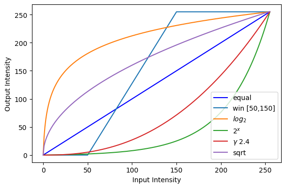

We saw previously that if our image has pixels that are all bunched up in color/intensity, leading to low contrast, our transfer function should accentuate those differences and thus improve contrast. We also saw how the histogram can tell us where to find these concentrations in the input domain.

Seen more practically then, a good transfer function has a slope above 1, leading to expansion and higher contrast, where the frequency of intensities is high in the input domain. To balance against that expansion though, the slope must end up less than 1, leading to compression of differences and reduction of contrast, in parts of the input domain that are sparsely populated.

As a result, we saw how an overexposed image, with many bright intensities and few dark ones, could be improved with for example an exponential ( $2^{x}$ ). Similarly an underexposed image, with large dark areas, could be improved by a $log$ or square root transform ( $\gamma=1/2$ ).

Make Gaussian and Uniform Random Images¶

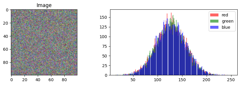
See how the uniform has better contrast, see what that means in the histograms. We can see that higher contrast goes in hand with a uniform histogram.

I_uniform = np.uint8(256*np.random.random((100,100,3)))
I_gauss = np.clip(128 + 30*np.random.randn(100,100,3), 0, 255).astype('uint8')

vis_hists(I_uniform)
vis_hists(I_gauss)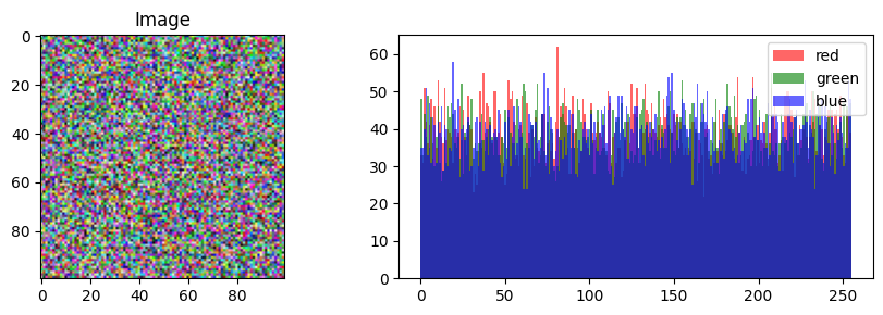

Build a parametric function that would spread the data out in `I_gauss`.¶

If we look at the above Gaussian distribution, and imagine drawing the transfer function over it, we can see that towards the extremes, where there’s not much data, the curve should be flat. Further, towards the middle the curve should be steep, to represent the idea that we are taking small differences in the input and mapping them to larger differences in the output.

This ends up looking something like an S curve or sigmoid.

S(x) = \frac{1}{1 + e^{-x}}

(1)

But we need a sigmoid that is centered around .5 and steep enough to look like an s inside [0,1]. We can rescale to our $[0,255]$ mapping afterwards.

S(x, x_c, s) = \frac{1}{1 + e^{-s(x-x_c)}}

(2)

def make_scurve(xc, s):
    return lambda x: 1/(1+np.exp(-(s*(x-xc))))

x = np.arange(0,1,1/100)
# f = lambda x: 1/(1+np.exp(-(10*(x-.5))))
f = make_scurve(.5, 10)
plt.figure(figsize=(4,3))
plt.plot(x, f(x));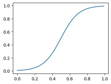

Apply the function to `I_gauss` and see how it improves contrast.¶

Since the S-curve function will return floating point numbers, for display purposes we must stick to $[0,1]$ .

vis_pair(I_gauss, f(I_gauss/255.0)) # or (255*f(I_gauss/255.0)).astype('uint8'))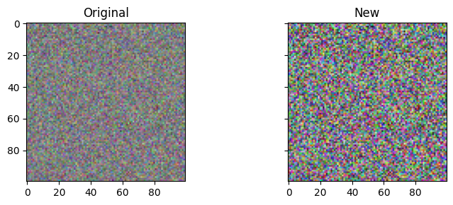

# vis_rgg_cube(I_gauss) # Comment in this line if you want to see the original I_gauss cube.
vis_rgb_cube(I_gauss/255.0)
vis_rgb_cube(f(I_gauss/255.0))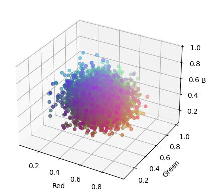

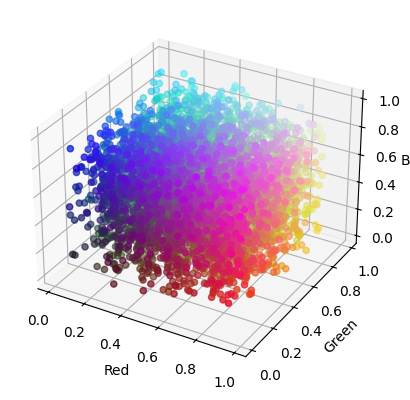
We can accomplish the same thing empirically, through the cumulative distribution function or CDF on the histogram¶

A fundamental result from probability theory, if $s = \mathbf{T}(r)$ for $\mathbf{T}$ continuous and differentiable:

p_s(s) = p_r(r)\begin{vmatrix}{\frac{dr}{ds}}\end{vmatrix}

(3)

The CDF measures the probability that a random variable $X$ takes on a value less than or equal to $x$ :

P(X \le x) = \intop_{0}^{x} p_r(w)dw

(4)

where $p_r$ is the probability distribution (read: histogram) of our random variable $r$ . So to transform into a uniform distribution, our transfer function should be:

s = \mathbf{T}(r) = (L-1) \intop_{0}^{r} p_r(w)dw

(5)

Another way of looking at this transfer function is that it transforms an input intensity to that intensity’s rank/percentile in the image (then scaled by the output max). For example, if a pixel is at least as bright as three-quarters of the image pixels in the input, then that pixel will have three-quarters of the max brightness in the output.

Lastly, you have likely run into a real-world analogy to the CDF, in the form of your standardized test scores. The CDF provides the conversion from your test score to your percentile ranking compared with all others who took the test.

Computing the CDF¶

This next cell is key step 1 in performing histogram equalization: We must compute the Cumulative Distribution Function (CDF), which once normalized is the transfer function we want to apply.

We use numpy.histogram to get frequency counts freq for each possible intensity. (In floating point data it’s not particularly different, it’s just that each bin will end up representing more than one discrete intensity).
We use numpy.cumsum to gives a rolling sum cdf of the frequency counts in freq. It’s just a list of all the intermediate sums on the way to the overall sum.
We normalize both freq and cdf. This happens to help for the purpose of visualizing the two together, but in the case of cdf we’ll see it also helps normalizing the output of the transfer function easier. We could just end up multiplying by our maximum brightness.

The slope of the CDF at any bin is now proportional to the number of pixels in that bin. And we know that in order to improve contrast in an image, we want the slope of our transfer function to be high in places where there are lots of pixels bunched up together in intensity. So there we have it: the CDF exhibits exactly the slope we need in order to improve contrast.

# First get the histogram of I_gauss, and plot with the cdf.
# normalize so they show up nicely.

bins=np.arange(257)
freq, bins = np.histogram(I_gauss.ravel(), bins=bins)
freq = freq/freq.max()
cdf = np.cumsum(freq)
cdf = cdf/cdf.max()

f = plt.figure(figsize=(4,3))
plt.bar(bins[:-1], freq, width=.5) # width to keep the bars skinny enough.
plt.plot(bins[:-1], cdf, 'b-', label='$CDF_{\mathtt{I\_gauss}}$');
plt.plot(x*255, make_scurve(.5, 10)(x), 'r-', label='S-curve');
plt.legend();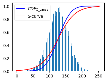

You can see in the above that indeed that the CDF has a high slope where there is a lot of data, and a lower slope where there is little or no data. It’s coincidental that the sigmoid can come close to matching the CDF of a Gaussian.

Now for key step 2 in performing histogram equalization: We must apply the cdf (coming from the histogram) as our transfer function.

For this we’re going to use the scipy function factory scipy.interpolate.interp1d. With the input range x coordinates bins and the output y values from cdf, interp1d returns a function that: given an $x'$ in the input range returns the value $y'$ through interpolation.

func = interp1d(bins[:-1], cdf, fill_value='extrapolate') 
# 'extrapolate' is important here, otherwise a lot of out of bound errors.

vis_pair(I_gauss, func(I_gauss), second_title='Hist Equalized')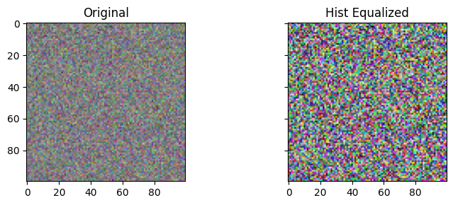

arr_info(func(I_gauss))

((100, 100, 3),
 dtype('float64'),
 np.float64(6.666666666666674e-05),
 np.float64(1.0))

Clearly the CDF does a decent job here of improving the contrast from the original. There’s also a bit of a matplotlib gotcha at work here: the histogram-equalized image is actually floating point in $[0,1]$ . If we wanted to convert back to integer, we must remember to multiply by 256 before casting to uint8.

As an aside: In that we have constructed I_gauss to be uint8 type integer data, we don’t actually need the interp1d we use above. A pixel value in I_gauss can serve perfectly well to simply index the cdf array. However the interp1d approach is generalizable to other kinds of image data, so I leave it here.

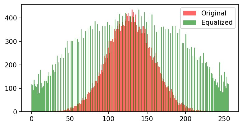
Let’s see what this did to our histogram. We’ll plot together the original and equalized images’ histograms to observe the difference directly.

# View the two histograms
f, axarr = plt.subplots(1,1, figsize=(6, 3))

funcI = func(I_gauss)

axarr.hist(I_gauss.ravel(), bins=bins, alpha = .6, label = 'Original', color = 'r');
axarr.hist(256*funcI.ravel(), bins=bins, alpha = .6, label = 'Equalized', color = 'g');
axarr.legend(loc = 'upper right');
plt.show()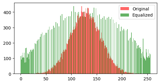

Conclusion¶

As you can see in this abstract example, histogram equalization is an ideal transfer function if the goal is to enhance the contrast in the image by making the histogram uniform, or as uniform as possible.

And here we get to the end of a notebook without having seen the application to any “real” natural image the kind about which we humans are concerned. Oh well, I leave it to you.

🔨 Your Turn: Equalize a Real Image¶

Task: Apply histogram equalization to a natural image, such as ../dip_pics/underExposed.jpg or ../dip_pics/got_tooDark.jpg, and show the original and equalized images side by side along with their histograms. Then do it a second way that leaves the colors alone, and compare.

Guidance:

It’s likely you can simply rename I_gauss and initialize it to plt.imread(...) for some image, then re-run the CDF cells. Check with arr_info that you have uint8 data in $[0,255]$ first.
Be careful though, as treating all channels as one distribution, as we’ve done here, can lead to the warping of color. This doesn’t have much of an effect in our example since the R,G,B channels all do come from the same Gaussian distribution. In natural images that’s less likely.
To address this, think of alternative colorspaces: equalize only a brightness channel, such as V in HSV or L in Lab, and leave the color channels alone. You’ll need a histogram and CDF of that channel’s own range rather than $[0,255]$ .
To check your work, the equalized histogram should be much flatter, and its CDF close to a straight line. You can also compare against skimage.exposure.equalize_hist.