Discrete Cosine Transform Introduction

stough 202-

Preview: Discrete Cosine Transform Introduction

Reading: DIP 6.6, 8.9

Throughout this BlockTransform module we have thought about how the numbers we use to describe an image can be more or less efficient based on whether each number represents a single pixel or a whole pattern within a image block. This pattern-based composition of an image can very powerful due to the fact of spatial coherence in the images about which we are concerned.

We saw in view_basis_blocks numerous useful basis patterns:

The Standard/Euclidean basis patterns show how we conceptualize an image being displayed, where every coefficient/number represents information about an individual pixel, and all pixels are independent.
The Haar basis patterns showed how we can decompose the energy within a block by representing instead the average of the block plus many larger- and smaller-scale differences from that average.

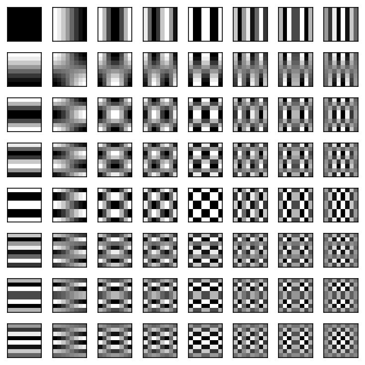
In this notebook we’ll look at another basis pattern that is so efficient for natural images (like those you might take with your camera) that it forms the basis for JPEG compression: the Discrete Cosine Transform.

Discrete Cosine transform matrix.¶

Each row of this matrix represents a sampled cosine wave with varying frequency over the signal space (s-D space, where s is the number of pixels). In that it satisfies the three conditions we specified previously (left to you to prove), it can serve just as well as either of the above two. It is based in Fourier analysis on the idea that any signal can be constructed from cosine and sine waveforms.

The DCT is even more powerful for natural images because unlike the Standard and Haar bases, here every basis pattern extends over the whole block. In fact, some form of DCT is usually so powerful, it has been adopted for use in JPEG, MPEG, and many other image and video compression standards.

Recall $s$ is the number of pixels, i.e. the size of our square matrix. The first row is again the mean, while later rows ( $u$ ) are sampled (by column $j$ ) cosines:

DCT_0 = \sqrt \frac{1}{s} \\ DCT_u = \sqrt \frac{2}{s}cos\Bigl(\frac{(2j+1)u\pi}{2s}\Bigr), j = 0,\dots,s-1, u = 1,\dots,s-1

%matplotlib inline
import matplotlib.pyplot as plt
import numpy as np

# For importing from alternative directory sources
import sys  
sys.path.insert(0, '../dip_utils')

from matrix_utils import (arr_info,
                          make_linmap)
from vis_utils import (vis_rgb_cube,
                       vis_hists,
                       vis_pair,
                       vis_surface)

from wavelet_utils import (make_haar_matrix,
                           make_random_basis,
                           make_klt_basis,
                           make_dct_matrix,
                           make_standard_matrix,
                           vis_blocks)

1. Start by plotting the relevant 2N-periodic cosine function (and remembering what such a thing is):¶

cos\Bigl(\frac{(2j+1)u\pi}{2s}\Bigr), j = 0,\dots,s-1, u = 1,\dots,s-1

N = 8 # or 16 or whatever
x = np.arange(0, 2*N, .01)
s = lambda x,u,N: np.cos(((2*x + 1)*u*np.pi)/(2*N))
plt.figure(figsize=(8,2))
plt.plot(x, s(x,0,N))

2. Add plots for additional values of u up to N-1 (just rerun the last line with different u) . Show.¶

3. On a relatively clean plot, with maybe just one or two of the above, additionally use plt.scatter and show the function values at integer x, as in: `xp = np.arange(0, 2*N)`¶

4. What does the below show (* is an element-wise multiply)?¶

print((s(x,1,8)*s(x,2,8)).sum())
print((s(x,4,8)*s(x,7,8)).sum())

Discrete Cosine transform matrix.¶

1. Start by plotting the relevant 2N-periodic cosine function (and remembering what such a thing is):¶

2. Add plots for additional values of u up to N-1 (just rerun the last line with different u) . Show.¶

3. On a relatively clean plot, with maybe just one or two of the above, additionally use plt.scatter and show the function values at integer x, as in: xp = np.arange(0, 2*N)¶

4. What does the below show (* is an element-wise multiply)?¶

5. Show plt.imshow(make_dct_matrix(8)))¶

3. On a relatively clean plot, with maybe just one or two of the above, additionally use plt.scatter and show the function values at integer x, as in: `xp = np.arange(0, 2*N)`¶

5. Show `plt.imshow(make_dct_matrix(8))`)¶