Intro to 2D PCA. - imageprocessing-awesome

stough 202-

Khan academy videos on Linear Algebra background.
Neat walkthrough for a simple example.

In the block transform chapter we re-expressed image blocks in terms of different bases (Haar, DCT, and others), and saw that a good basis packs most of a block’s energy into just a few coefficients. Those bases were fixed in advance, the same for every image. Principal Component Analysis (PCA) asks: what is the best basis for this particular data? PCA finds the orthogonal directions along which the data varies the most, ordered from most variance to least. Keep only the first few directions and you have the most faithful low-dimensional summary of the data possible with a linear basis. (In signal processing the same idea is called the Karhunen-Loève Transform, KLT; make_klt_basis in wavelet_utils is exactly this.)

We’ll start in 2D, where we can see everything, with data whose answer we know in advance.

%matplotlib inline
import matplotlib.pyplot as plt
import numpy as np
from sklearn.decomposition import PCA

Generate Some Random Data.¶

X = np.array([4,6], ndmin=2).T + np.random.randn(2,500)

def gen_pca_data(mu=[10,20], var=[6,1], evs=[[1,1], [1,-1]], num=500):
    # Gaussian Normal axis-oriented data scaled by the variance.
    X = np.sqrt(np.array(var)[:,None])*np.random.randn(len(mu),num)

    # norm the row vectors: https://necromuralist.github.io/neural_networks/posts/normalizing-with-numpy/
    evs = evs/np.linalg.norm(evs, ord=2, axis=1, keepdims=True)

    # Apply the row vectors as a rotation, to reorient the data
    X = np.matmul(evs, X)

    # Add back in the mean
    X = np.array(mu, ndmin=2).T + X
    
    return X.T

X = gen_pca_data()

gen_pca_data builds data with a known structure. It draws 500 points from an axis-aligned 2D Gaussian with variance 6 along the first axis and 1 along the second. Then it rotates them so those axes point along the directions $\langle 1, 1 \rangle$ and $\langle 1, -1 \rangle$ , normalized to unit length, and shifts the whole cloud to be centered at $(10, 20)$ . (The first line of the cell above, making X from [4,6], is immediately replaced, so it has no effect.) So if PCA works, it should tell us: mean about $(10,20)$ , variances about 6 and 1, and directions about $\pm\frac{1}{\sqrt{2}}\langle 1, 1 \rangle$ and $\pm\frac{1}{\sqrt{2}}\langle 1, -1 \rangle$ .

plt.figure(figsize=(4,4))
plt.scatter(X[:,0], X[:,1], edgecolors='k', alpha=.25)
plt.scatter([0],[0], color='r', marker='+');
plt.axis('equal');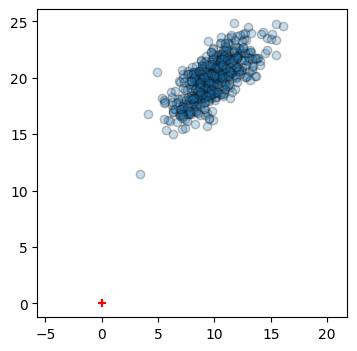

PCA will find directions in the data space that account for the most variance.¶

pca = PCA(n_components=2)
Xt = pca.fit_transform(X)

print(f'PCA found MEAN: {pca.mean_}')
print(f'          VAR : {pca.explained_variance_}')
print(f'components    : \n{pca.components_}')

PCA found MEAN: [ 9.83915171 19.93707048]
          VAR : [6.50879959 1.04940098]
components    : 
[[ 0.724062   0.6897349]
 [-0.6897349  0.724062 ]]

Just what we built in, up to sampling noise from having only 500 points. The mean is about $(10, 20)$ , the variances about 6 and 1, and the rows of components_ are the two diagonal directions, each with entries of about $0.707 = \frac{1}{\sqrt{2}}$ . (PCA can’t tell a direction from its opposite, so either one may come out with its sign flipped.)

Where do the components come from?¶

PCA computes the covariance matrix of the data,

\mathbf{C} = \frac{1}{n-1}\sum_{i=1}^{n} (\mathbf{x}_i - \boldsymbol{\mu})(\mathbf{x}_i - \boldsymbol{\mu})^\intercal

whose diagonal holds the variance of each coordinate and whose off-diagonal entries hold how the coordinates vary together. The principal components are the eigenvectors of $\mathbf{C}$ , and the variance along each is its eigenvalue. Since $\mathbf{C}$ is symmetric, its eigenvectors are orthogonal, so they form a new orthonormal basis, a rotation of the original axes. Let’s confirm that sklearn is doing exactly this:

C = np.cov(X.T)
evals, evecs = np.linalg.eigh(C)       # eigh: for symmetric matrices; ascending order
order = np.argsort(evals)[::-1]        # largest variance first

print(f'covariance matrix:\n{C}\n')
print(f'eigenvalues : {evals[order]}')
print(f'eigenvectors (as rows):\n{evecs[:, order].T}')

covariance matrix:
[[3.91157681 2.72648277]
 [2.72648277 3.64662375]]

eigenvalues : [6.50879959 1.04940098]
eigenvectors (as rows):
[[-0.724062  -0.6897349]
 [ 0.6897349 -0.724062 ]]

Same variances, same directions (again, possibly with signs flipped). Notice the covariance matrix itself: its large off-diagonal entries say that the two coordinates are strongly correlated. In the PCA coordinates, that correlation is gone. Let’s check the covariance of the transformed data Xt:

np.cov(Xt.T).round(3)

array([[ 6.509, -0.   ],
       [-0.   ,  1.049]])

Diagonal: in the new basis the coordinates are uncorrelated, and all the variance has been sorted into the first coordinate as much as possible. This is the same “energy compaction” we wanted from block transforms, but here the basis is tailored to the data.

Plot with the PCA directions.¶

Each dashed line runs from $-3\sigma$ to $+3\sigma$ along a principal direction, centered on the mean (orange), where $\sigma$ is the standard deviation along that direction. Nearly all the data falls within these lines.

plt.figure(figsize=(4,4))

# Data and origin
plt.scatter(X[:,0], X[:,1], color = 'gray', edgecolors='k', alpha=.25)
plt.scatter([0],[0], color='r', marker='+');

# mean
plt.scatter(pca.mean_[0], pca.mean_[1], color='orange')

# pca lines, +- 3 sigma
sigmas = np.sqrt(pca.explained_variance_)
pca0 = np.array([pca.mean_ - 3*sigmas[0]*pca.components_[0,:], pca.mean_ + 3*sigmas[0]*pca.components_[0,:]])
pca1 = np.array([pca.mean_ - 3*sigmas[1]*pca.components_[1,:], pca.mean_ + 3*sigmas[1]*pca.components_[1,:]])

plt.plot(pca0[:,0], pca0[:,1], 'c--', linewidth=3)
plt.plot(pca1[:,0], pca1[:,1], 'r--', linewidth=3);
plt.axis('equal');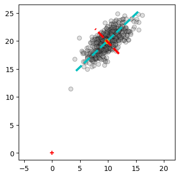

Let’s reconstruct¶

Very similar to the reconstruction we’ve done in the past with respect to DCT and Haar. Just more general.

Each point is just the mean + sum(coeff*component for every transform coefficient):

\mathbf{x} = \boldsymbol{\mu} + \sum_k c_k \mathbf{v}_k, \qquad c_k = \mathbf{v}_k \cdot (\mathbf{x} - \boldsymbol{\mu})

where the $\mathbf{v}_k$ are the components. The coefficients $c_k$ are exactly what fit_transform gave us in Xt: each is the projection (dot product) of the mean-centered point onto one component.

print(f"We'll here attempt to reconstruct \n"
      f"the point {X[0,:]} from its \n"
      f"transform {Xt[0,:]}.")

We'll here attempt to reconstruct 
the point [ 8.60521937 20.56572036] from its 
transform [-0.45984176  1.30626768].

print('Recall')
print(f'PCA is MEAN: {pca.mean_}')
print(f'       VAR : {pca.explained_variance_}')
print(f'components : \n{pca.components_}')

Recall
PCA is MEAN: [ 9.83915171 19.93707048]
       VAR : [6.50879959 1.04940098]
components : 
[[ 0.724062   0.6897349]
 [-0.6897349  0.724062 ]]

tp = Xt[0,:]  # transform point.

print('The reconstruction is \n'
      f'     {pca.mean_} \n'
      f'plus {tp[0]}*{pca.components_[0,:]}\n'
      f'plus {tp[1]}*{pca.components_[1,:]}')

The reconstruction is 
     [ 9.83915171 19.93707048] 
plus -0.4598417602677216*[0.724062  0.6897349]
plus 1.306267682788583*[-0.6897349  0.724062 ]

# Add first component
rp = pca.mean_ + tp[0]*pca.components_[0,:]
print(f'rp is {rp} after the first component.')

# Add second component
rp += tp[1]*pca.components_[1,:]
print(f'rp is {rp} after the second component.\n')

print(f'So, pretty close to {X[0,:]}')

rp is [ 9.50619777 19.61990157] after the first component.
rp is [ 8.60521937 20.56572036] after the second component.

So, pretty close to [ 8.60521937 20.56572036]

With both components we recover the point exactly. The interesting question is what happens with fewer.

Dimensionality reduction¶

Let’s reconstruct every point using only the first component, $\mathbf{x} \approx \boldsymbol{\mu} + c_0 \mathbf{v}_0$ . That’s describing each 2D point with a single number.

X1 = pca.mean_ + np.outer(Xt[:,0], pca.components_[0,:])   # one coefficient per point

plt.figure(figsize=(4,4))
plt.scatter(X[:,0], X[:,1], color='gray', edgecolors='k', alpha=.25, label='original')
plt.scatter(X1[:,0], X1[:,1], color='c', s=8, label='1-component reconstruction')
plt.legend(fontsize=8)
plt.axis('equal');

err = np.mean(np.sum((X - X1)**2, axis=1))
print(f'mean squared reconstruction error: {err:.3f}')
print(f'variance along the dropped component: {pca.explained_variance_[1]:.3f}')
print(f'fraction of variance kept: {pca.explained_variance_ratio_[0]:.3f}')

mean squared reconstruction error: 1.047
variance along the dropped component: 1.049
fraction of variance kept: 0.861

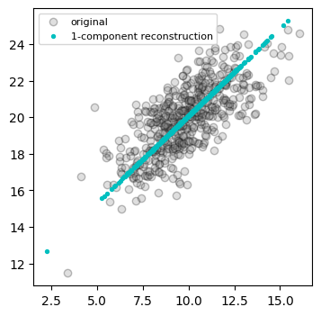
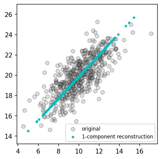
Every point collapses onto the first principal line, its orthogonal projection. The error we make is exactly what we threw away: the mean squared error equals the variance along the dropped second component, up to the $n$ versus $n-1$ in the variance formula. With one number per point instead of two, we keep about $\frac{6}{7}$ of the variance.

No other single direction would do better. That’s the defining property of PCA: for any number of components $k$ , the first $k$ principal components give the smallest possible mean squared reconstruction error among all $k$ -dimensional linear approximations. In 2D this is a curiosity. With images of faces or handwritten digits, with thousands of pixels each, it’s a powerful way to find the few directions that matter.