Convolutional NN on Yale Face Database B with torch

stough 202-

Preview: Convolutional NN on [Yale Face Database B](http://vision.ucsd.edu/~iskwak/ExtYaleDatabase/ExtYaleB.html) with [torch](https://pytorch.org/)

Trying to recognize faces under variable lighting.

This is face recognition as a classification problem: given a cropped photo, which of the 38 people is it? It follows the same recipe as the MNIST convolutional network, with bigger images ( $192 \times 168$ ), more classes, far fewer examples per class (about 58 training photos per person), and the dramatic lighting changes we saw while exploring the data.

%matplotlib inline
# or widget
import matplotlib.pyplot as plt

import numpy as np
import copy
import tempfile

from functools import partial
from multiprocessing.pool import ThreadPool

# from keras.datasets import mnist
import torchvision
from torchvision import datasets, transforms
from torchvision.datasets import ImageFolder
from torchvision.utils import make_grid
from torch.utils.data import (Dataset, 
                              DataLoader,
                              random_split)
from torch.optim.lr_scheduler import StepLR

# torch
import torch
import torch.optim as optim
import torch.backends.cudnn as cudnn

import torch.nn.functional as F

from torch import nn
from torch.autograd import Variable
from torch.nn import Module

# For timing.
import time
tic, toc = (time.time, time.time)

# For importing from alternative directory sources
import sys
sys.path.insert(0, '../dip_utils')
from data_paths import yale_root
from torch_utils import train, test

Namespace for parameters.¶

The same settings Namespace as in the linear model, where it’s explained.

from argparse import Namespace
# What is a Namespace? It looks like this. 
# Such objects allow you to use the dot operator, like a struct in C.
# class Namespace:
#     def __init__(self, **kwargs):
#         self.__dict__.update(kwargs)

args = Namespace(
    no_cuda=False, 
    seed=1, 
    batch_size=32,
    test_batch_size=100,
    epochs=20,
    lr=1.0,
    gamma=0.8,
    log_interval=30,
    save_model=False,
    trainSize=.9
)

Organize the Face data¶

We’ll use the torchvision ImageFolder to automatically make a dataset from the face data folder. Then we’ll randomly split the dataset into 90% training and 10% test using random_split. The split is random but seeded, with its own generator, so that it’s the same photos in each set on every run, and results can be compared from run to run.

yaleData = ImageFolder(yale_root(), 
                       transform=transforms.Compose([
                           transforms.Grayscale(),
                           transforms.Resize((192,168), interpolation=torchvision.transforms.InterpolationMode.BILINEAR),
                           # Random recolorization every load, for the training AND test images (see below).
                           # For a consistent test set, delete this line (losing the augmentation), or
                           # load the data twice, with and without it, and split both the same way.
                           transforms.ColorJitter(brightness=.5, contrast=.3),
                           transforms.ToTensor()
                       ]))

NUMCLASSES = len(yaleData.classes)

split_lengths = np.round([f*len(yaleData) for f in [args.trainSize, 1-args.trainSize]]).astype(np.int32).tolist()
# Seed the split, so that every run trains and tests on the same photos.
trainFaces, testFaces = torch.utils.data.random_split(yaleData, split_lengths,
                                                      generator=torch.Generator().manual_seed(42))

One subtlety: random_split makes trainFaces and testFaces views of the same yaleData, so they share its transform, including the random ColorJitter. That means the test images are also randomly re-jittered every time they’re loaded, so the test accuracy will wobble a little from epoch to epoch for reasons that have nothing to do with the model. A cleaner setup would load the data twice, with jitter for training and without it for testing, and split both the same way.

Explore the data a bit.¶

trainFaces and testFaces are both subsets of the yaleData Dataset. They implement __len__ and __getitem__, so look at what some of the elements are.

# Here, let's view some random faces
samples = torch.stack([testFaces[i][0] 
                       for i in np.random.choice(len(testFaces), 64, replace=False)])
plt.figure(figsize=(5,5))
plt.imshow(make_grid(samples, nrow=8, pad_value=1.0).permute(1,2,0))
plt.tight_layout()

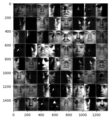
# Here, see how the same face is changed each time due to the ColorJitter.
samples = torch.stack([testFaces[101][0] 
                       for i in range(64)])
plt.figure(figsize=(5,5))
plt.imshow(make_grid(samples, nrow=8, pad_value=1.0).permute(1,2,0))
plt.tight_layout()

# Here, let's count how many examples of each person shows up in the data overall.
import pandas
pandas.Series([yaleData.classes[tup[1]] for tup in trainFaces]).value_counts()

Make the DataLoaders that we’ll use.¶

use_cuda = not args.no_cuda and torch.cuda.is_available()
torch.manual_seed(args.seed)
device = torch.device("cuda" if use_cuda else "cpu")

kwargs = {'num_workers': 4, 'pin_memory': False} if use_cuda else {}

train_loader = torch.utils.data.DataLoader(trainFaces,
    batch_size=args.batch_size, shuffle=True, **kwargs)
test_loader = torch.utils.data.DataLoader(testFaces,
    batch_size=args.test_batch_size, shuffle=False, **kwargs)

Define the Network¶

Use Convolutional Layers to transform the original image into a collection of features that linear layers can use to discriminate among the classes.

To keep all the layers’ dimensions in agreement, take a look at the prime factorizations of your image dimesions.

168 = 2 x 2 x 2 x 3 x 7
192 = 2 x 2 x 2 x 2 x 2 x 2 x 3

Tracing the shapes: a $3 \times 3$ convolution with padding=2 actually grows each dimension by 2, and padding=1 keeps it the same; each max pool halves it (rounding down). So $192 \times 168$ becomes $194 \times 170 \to 97 \times 85 \to 99 \times 87 \to 49 \times 43 \to 49 \times 43 \to 24 \times 21$ , and the 64 feature maps of $24 \times 21$ flatten to $64 \cdot 24 \cdot 21 = 32256$ inputs for fc1.

The network returns raw class scores (logits), not probabilities. F.cross_entropy applies the softmax itself.

A cautionary tale. An earlier version of this network ended with output = torch.sigmoid(x), and you’ll find that line commented out at the end of forward. It looks harmless, and the network still trains and runs without any error. But cross-entropy applies a softmax to whatever it’s given, $p_k = e^{s_k} / \sum_j e^{s_j}$ , and a sigmoid has already squashed every score $s_k$ into $(0, 1)$ . With 38 classes, the best the correct class can then do is $p = e / (e + 37) \approx 0.07$ , so the loss can never fall below $-\ln 0.07 \approx 2.7$ , and the gradients that should push the right answer up stay weak. One extra line quietly ruins the outcome. For how softmax and cross-entropy work together, see the softmax classifier notes from Stanford’s CS231n.

class Net(nn.Module):
    def __init__(self):
        super(Net, self).__init__()
        self.conv1 = nn.Conv2d(1, 8, 3, 1, padding=2) # keep the size 
        self.conv2 = nn.Conv2d(8, 16, 3, 1, padding=2)
        # pool 4x4 here.
        self.conv3 = nn.Conv2d(16, 32, 3, 1, padding=1)
        self.conv4 = nn.Conv2d(32, 64, 3, 1, padding=1)
        # pool 2x2 here
        
        self.dropout1 = nn.Dropout2d(0.25)
        self.dropout2 = nn.Dropout2d(0.5)
        self.fc1 = nn.Linear(32256, 256)
        self.fc2 = nn.Linear(256, NUMCLASSES)

    def forward(self, x):
        x = self.conv1(x) 
        x = F.relu(x)
        x = F.max_pool2d(x, 2) 
        
        x = self.conv2(x) 
        x = F.relu(x)
        x = F.max_pool2d(x, 2) 
        
        x = self.conv3(x)
        x = F.relu(x)
        x = self.conv4(x)
        x = F.relu(x)
        x = F.max_pool2d(x, 2) # outputs are 24x21
        
#         x = self.dropout1(x) # randomly zero out some of the features. (in training only)
        x = torch.flatten(x, 1)  
        x = self.fc1(x) 
        x = F.relu(x)
#         x = self.dropout2(x)
        x = self.fc2(x)
        # output = torch.sigmoid(x)  # Don't: see "A cautionary tale" above.
        # Return raw scores (logits): F.cross_entropy applies its own softmax.
        output = x
        return output

Training and Test functions.¶

train and test are the same loops we wrote out and walked through step by step in the linear model. Every network in this chapter trains and tests the same way, so rather than repeat them in each notebook, they now live in torch_utils and are imported at the top, just as arr_info moved to matrix_utils after the numpy tutorial. Two small differences from the inline version: they take the loss function as an argument (loss_fn), and they return the losses and accuracy so that we can plot the training curves. The file is short; open it and read it once.

This network returns raw scores, so its loss is F.cross_entropy, which applies the softmax for us.

Instantiate the model and count parameters¶

model = Net().to(device)
# Count the number of parameters: 
print(f'model has {sum(p.numel() for p in model.parameters() if p.requires_grad)} parameters.')

Run the optimization¶

# optimizer = optim.Adadelta(model.parameters(), lr=args.lr)
optimizer = optim.Adam(model.parameters())
scheduler = StepLR(optimizer, step_size=1, gamma=args.gamma)

test_loss = []
test_acc = []
train_loss = []

for epoch in range(1, args.epochs + 1):
    train_loss.append(train(args, model, device, train_loader, optimizer, epoch, loss_fn=F.cross_entropy))
    results = test(args, model, device, test_loader, loss_fn=F.cross_entropy)
    test_loss.append(results[0])
    test_acc.append(results[1])
    scheduler.step()

if args.save_model:
    torch.save(model.state_dict(), "faces_cnn.pth")

...
Train set: Average loss: 0.0217 (1.603 sec)
Test set: Average loss: 0.1040, Accuracy: 241/245 (98%)
Train Epoch: 19 [0/2207 (0%)]	Loss: 0.035926
Train Epoch: 19 [960/2207 (43%)]	Loss: 0.000376
Train Epoch: 19 [1920/2207 (87%)]	Loss: 0.000286
Train set: Average loss: 0.0216 (1.598 sec)
Test set: Average loss: 0.0869, Accuracy: 242/245 (99%)
Train Epoch: 20 [0/2207 (0%)]	Loss: 0.000431
Train Epoch: 20 [960/2207 (43%)]	Loss: 0.002463
Train Epoch: 20 [1920/2207 (87%)]	Loss: 0.001132
Train set: Average loss: 0.0217 (1.604 sec)
Test set: Average loss: 0.0871, Accuracy: 242/245 (99%)

# https://matplotlib.org/gallery/api/two_scales.html

train_loss = np.array(train_loss)
test_loss = np.array(test_loss)
test_acc = np.array(test_acc)

fig, ax1 = plt.subplots()
ax1.plot(np.stack([train_loss, test_loss]).T);

ax2 = ax1.twinx()
ax2.plot(test_acc, 'r--', label='test_acc');


ax1.legend(labels=['train_loss', 'test_loss'], loc='upper left')
ax2.legend(loc='upper right');

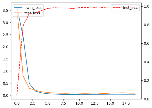
Losses (left axis) and test accuracy (right axis, dashed) by epoch. With only about 2,200 training photos, watch for the two loss curves separating: training loss that keeps falling while test loss levels off or rises is the signature of overfitting, memorizing the training photos rather than learning what distinguishes faces. That’s what happens here: within a few epochs the training loss falls to nearly zero, while the test loss levels off (around 0.1 to 0.15) and test accuracy plateaus near 98%. (Small differences remain from run to run, from the random ColorJitter and the GPU’s arithmetic.) The dropout layers defined in Net are commented out in forward; try enabling them and compare.

Let’s get the output of the model for all the test data.¶

The test_loader isn’t shuffled, but we’ll still keep track of the targets alongside the outputs, to know what the answer should have been. In fact, let’s just keep all of it.

In the below cell we loop over all the test data, push it through the model and store the resulting classifier outputs. The expression model(data.to(device)) sends the data to the GPU (where the model resides) and applies the model to it. The sequence that happens after, .cpu().detach().numpy(), takes the resulting outputs and brings it back to the cpu memory space in the form of a numpy array.

A notes on pretty-printing arrays.

model.eval() # make sure the model weights don't change.
outputs = np.concatenate([model(data.to(device)).cpu().detach().numpy() 
              for data, target in test_loader], axis=0)

outputs[0]

predicted = np.argmax(outputs, axis=1)

target = np.concatenate([target for data, target in test_loader], axis=0)

wrongs = np.nonzero(predicted != target)[0]

len(wrongs)/len(test_loader.dataset)

len(wrongs), len(test_loader.dataset)

# The misclassified test faces (if there are any!)
samples = torch.stack([testFaces[i][0] 
                       for i in wrongs]) if len(wrongs) else torch.zeros(1, 1, 192, 168)
plt.figure(figsize=(5,3))
plt.imshow(make_grid(samples, nrow=5, pad_value=1.0).permute(1,2,0))
plt.tight_layout()

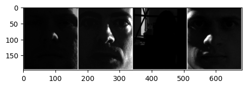
print('Predicted: ' + ' '.join(['%02d' % x for x in predicted[wrongs]]))
print('Actual:    ' + ' '.join(['%02d' % x for x in target[wrongs]]))

Look at which test faces were misclassified. Nearly all of them are photos with the most extreme lighting: half in shadow, or nearly black. In those images little of the face is visible at all. Considering how differently the same person can look across these photos, it’s remarkable how well a small network does with fewer than 60 examples per person.