Convolutional NN on MNIST with torch - imageprocessing-awesome

stough 202-

Preview: Convolutional NN on [MNIST](https://github.com/pytorch/examples/tree/master/mnist) with [torch](https://pytorch.org/)

Following a simple digit classification on MNIST, using a small convolutional neural network (CNN).

A convolutional layer solves for simple spatial filtering operations where the output (feature map) contains useful information for the downstream or deeper layers in the network. With $in\_channels$ input channels, $out\_channels$ output feature maps, and $kernel\_size$ for the filtering, the layer will have $in\_channels * out\_channels * kernel\_size^2 + out\_channels$ parameters to optimize.

%matplotlib inline
# or widget
import matplotlib.pyplot as plt

import numpy as np
from random import shuffle
import copy
import tempfile

# from keras.datasets import mnist
from torchvision import datasets, transforms
from torch.utils.data import Dataset, DataLoader
from torch.optim.lr_scheduler import StepLR

# torch
import torch
import torch.optim as optim
import torch.backends.cudnn as cudnn

import torch.nn.functional as F

from torch import nn
from torch.autograd import Variable
from torch.nn import Module

from torchvision.transforms import ToTensor
from torchvision.utils import make_grid

# For timing.
import time
tic, toc = (time.time, time.time)

# For importing from alternative directory sources
import sys
sys.path.insert(0, '../dip_utils')
from data_paths import mnist_root
from torch_utils import train, test

Define the Network¶

A more complicated network, using Convolutional Layers to transform the original image into a collection of features that a linear layer can use to discriminate among the classes/digits.

Layer by layer, for one $1 \times 28 \times 28$ input image:

conv1: 32 learned $3 \times 3$ filters, each correlated with the image, exactly like the spatial filters we designed by hand, except that training picks the weights. Output: 32 feature maps of $26 \times 26$ (no padding, so we lose a pixel at each border).
ReLU, $\max(0, x)$ : keeps positive responses and zeros out negative ones. Without a nonlinearity between them, two linear layers would collapse into one.
conv2: 64 filters, each $3 \times 3$ across all 32 feature maps, so each looks at combinations of the first layer’s features. Output: $64 \times 24 \times 24$ .
Max pooling: keep the largest value in each $2 \times 2$ block, halving the resolution to $64 \times 12 \times 12$ . This makes the features a little tolerant of small shifts.
Dropout: during training only, randomly zero a fraction of the values, so the network can’t rely too heavily on any one feature. This reduces overfitting.
fc1, fc2: flatten the $64 \cdot 12 \cdot 12 = 9216$ features and finish with two fully-connected layers, ending in 10 class scores and log_softmax, as in the linear model.

class Net(nn.Module):
    def __init__(self):
        super(Net, self).__init__()
        self.conv1 = nn.Conv2d(1, 32, 3, 1) # padding is 0 by default, so 
                                            # we lose a pixel on each side.
        self.conv2 = nn.Conv2d(32, 64, 3, 1)
        self.dropout1 = nn.Dropout2d(0.25)
        self.dropout2 = nn.Dropout(0.5)
        self.fc1 = nn.Linear(9216, 128)
        self.fc2 = nn.Linear(128, 10)

    def forward(self, x):
        x = self.conv1(x) # input: 1x28x28, output: 32x26x26
        x = F.relu(x)
        x = self.conv2(x) # input: 32x26x26, output: 64x24x24
        x = F.relu(x)
        x = F.max_pool2d(x, 2) # input: 64x24x24, output: 64x12x12
        x = self.dropout1(x) # randomly zero out some of the features. (in training only)
        x = torch.flatten(x, 1) # flatten the 64x12x12 to a single dimension (9216) 
        x = self.fc1(x) 
        x = F.relu(x)
        x = self.dropout2(x)
        x = self.fc2(x)
        output = F.log_softmax(x, dim=1)
#         output = torch.sigmoid(x)
        return output

Training and Test functions.¶

train and test are the same loops we wrote out and walked through step by step in the linear model. Every network in this chapter trains and tests the same way, so rather than repeat them in each notebook, they now live in torch_utils and are imported at the top, just as arr_info moved to matrix_utils after the numpy tutorial. Two small differences from the inline version: they take the loss function as an argument (loss_fn), and they return the losses and accuracy so that we can plot the training curves. The file is short; open it and read it once.

During training, the optimizer modifies the parameters of the model in a way that minimizes the loss function. See more detail here, but a lot is hidden from you. Just viewing it pythonically for example, it is not clear how the loss and the optimizer are connected.

This network ends in log_softmax, like the linear model, so its loss is F.nll_loss.

Namespace to replace the argparse business¶

The same settings Namespace as in the linear model, where it’s explained.

from argparse import Namespace
# What is a Namespace? It looks like this. 
# Such objects allow you to use the dot operator, like a struct in C.
# class Namespace:
#     def __init__(self, **kwargs):
#         self.__dict__.update(kwargs)

args = Namespace(
    no_cuda=False, 
    seed=1, 
    batch_size=64,
    test_batch_size=1000,
    epochs=5,
    lr=1.0,
    gamma=0.7,
    log_interval=250,
    save_model=False
)

Organize the MNIST data¶

We’ll use the torchvision transforms to modify the dataset without having to convert to numpy arrays ourselves. If organized correctly, we won’t need our own custom DataLoader. That might come later.

Note also that the below code downloads the dataset into your data folder (~/data by default; see data_paths) the first time.

Normalize((0.1307,), (0.3081,)) subtracts MNIST’s mean pixel value and divides by its standard deviation, so the inputs are centered near 0 with spread about 1. Networks train more easily on inputs of that scale.

# Thank you: https://www.aiworkbox.com/lessons/load-mnist-dataset-from-pytorch-torchvision
# https://pytorch.org/vision/stable/datasets.html
mnist_trainset = datasets.MNIST(root=mnist_root(), train=True, download=True, 
                                transform=transforms.Compose([
                                    transforms.ToTensor(),
                                    transforms.Normalize((0.1307,), (0.3081,))
                                ]))
mnist_testset = datasets.MNIST(root=mnist_root(), train=False, download=True, 
                               transform=transforms.Compose([
                                   transforms.ToTensor(),
                                   transforms.Normalize((0.1307,), (0.3081,))
                               ]))

use_cuda = not args.no_cuda and torch.cuda.is_available()
torch.manual_seed(args.seed)
device = torch.device("cuda" if use_cuda else "cpu")

kwargs = {'num_workers': 4, 'pin_memory': False} if use_cuda else {}

train_loader = torch.utils.data.DataLoader(mnist_trainset,
    batch_size=args.batch_size, shuffle=True, **kwargs)
test_loader = torch.utils.data.DataLoader(mnist_testset,
    batch_size=args.test_batch_size, shuffle=False, **kwargs)

# If use_cuda is True, then we should be able to use the local GPU.
print(use_cuda, device)

Instantiate the model and count parameters¶

model = Net().to(device)
# Count the number of parameters: 
print(f'model has {sum(p.numel() for p in model.parameters() if p.requires_grad)} parameters.')

model

# Is the model actually on the GPU?
# Thanks: https://discuss.pytorch.org/t/how-to-check-if-model-is-on-cuda/180
next(model.parameters()).is_cuda

About 1.2 million parameters, compared to 7,850 for the linear model. Look at where they are: the two convolutional layers have only $32 \cdot (9+1) = 320$ and $64 \cdot (32 \cdot 9 + 1) = 18{,}496$ , because each small filter is reused at every position in the image. Nearly all the rest, $9216 \cdot 128 + 128 = 1{,}179{,}776$ , are in fc1. Weight sharing is what makes convolutional layers so economical.

Run the optimization¶

optimizer = optim.Adadelta(model.parameters(), lr=args.lr)
scheduler = StepLR(optimizer, step_size=1, gamma=args.gamma)

test_loss = []
test_acc = []
train_loss = []

for epoch in range(1, args.epochs + 1):
    train_loss.append(train(args, model, device, train_loader, optimizer, epoch, loss_fn=F.nll_loss))
    results = test(args, model, device, test_loader, loss_fn=F.nll_loss)
    test_loss.append(results[0])
    test_acc.append(results[1])
    scheduler.step()

if args.save_model:
    torch.save(model.state_dict(), "mnist_cnn.pth")

...
Train Epoch: 4 [0/60000 (0%)]	Loss: 0.245216
Train Epoch: 4 [16000/60000 (27%)]	Loss: 0.012227
Train Epoch: 4 [32000/60000 (53%)]	Loss: 0.004069
Train Epoch: 4 [48000/60000 (80%)]	Loss: 0.057392
Train set: Average loss: 0.0500 (4.637 sec)
Test set: Average loss: 0.0325, Accuracy: 9889/10000 (99%)
Train Epoch: 5 [0/60000 (0%)]	Loss: 0.008672
Train Epoch: 5 [16000/60000 (27%)]	Loss: 0.003186
Train Epoch: 5 [32000/60000 (53%)]	Loss: 0.030274
Train Epoch: 5 [48000/60000 (80%)]	Loss: 0.027037
Train set: Average loss: 0.0433 (4.684 sec)
Test set: Average loss: 0.0312, Accuracy: 9895/10000 (99%)

# https://matplotlib.org/gallery/api/two_scales.html

train_loss = np.array(train_loss)
test_loss = np.array(test_loss)
test_acc = np.array(test_acc)

fig, ax1 = plt.subplots()
ax1.plot(np.stack([train_loss, test_loss]).T);

ax2 = ax1.twinx()
ax2.plot(test_acc, 'r--', label='test_acc');


ax1.legend(labels=['train_loss', 'test_loss'], loc='upper left')
ax2.legend(loc='upper right');

# plt.savefig('../dip_outs/conv_MNIST_torch_training.png', dpi=300)

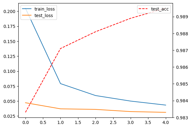
Losses (left axis) and test accuracy (right axis, dashed) after each epoch. Test accuracy reaches about 99% within a few epochs, versus about 92% for the linear model: roughly an eight-fold reduction in errors. The training loss stays a little above the test loss. That’s not a bug: dropout is active during training and switched off for testing, and the training loss is averaged over an epoch during which the model was still improving.

Let’s get the output of the model for all the test data.¶

Since the test_loader is also shuffled, we’re going to want to keep track of the target too, to know what the answer should have been. In fact, let’s just keep all of it.

In the below cell we loop over all the test data, push it through the model and store the resulting classifier outputs. The expression model(data.to(device)) sends the data to the GPU (where the model resides) and applies the model to it. The sequence that happens after, .cpu().detach().numpy(), takes the resulting outputs and brings it back to the cpu memory space in the form of a numpy array.

A notes on pretty-printing arrays.

model.eval() # make sure the model weights don't change.
outputs = np.concatenate([model(data.to(device)).cpu().detach().numpy() 
              for data, target in test_loader], axis=0)

outputs[0]

# The last function in the model is a log_softmax, which is a log after softmax.
# Softmax makes the outputs all in [0,1] and sum to 1, but then there is a log 
# after that. So we undo that to see the [0,1] numbers, which can be thought of 
# as probabilities.
with np.printoptions(precision=4, suppress=True):
    print(np.exp(outputs[0]))

Just for fun, let’s see some of the mistakes...¶

correct_labels = np.concatenate([target for data, target in test_loader], axis=0)

correct_labels.shape

proposed_labels = np.argmax(outputs, axis=-1)

proposed_labels.shape

sum(proposed_labels == correct_labels)

wrong_guesses = np.where(proposed_labels != correct_labels)[0]

wrong_guesses

from torchvision.utils import make_grid

which_wrong = np.random.choice(wrong_guesses, 64, replace=False)
samples = torch.stack([mnist_testset[r][0]
                       for r in which_wrong])
plt.imshow(make_grid(samples, nrow=8, pad_value=1.0).permute(1,2,0))

print('Predicted: ' + ' '.join(['%d' % x for x in proposed_labels[which_wrong]]))
print('Actual:    ' + ' '.join(['%d' % x for x in correct_labels[which_wrong]]))

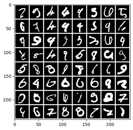
Look through these mistakes. Many are digits a person might hesitate over too: a 4 that’s nearly a 9, a 7 with an extra stroke, a 5 written like a 6, or digits that are cut off or smudged. A few are just strange, and some may arguably be labeled wrong. With only about 100 errors in 10,000, what’s left is mostly genuinely ambiguous handwriting.

print('\n'.join([str((x,y)) for x,y in zip(proposed_labels[which_wrong], correct_labels[which_wrong])]))