Linear MNIST with torch - imageprocessing-awesome

stough 202-

Preview: Linear [MNIST](https://github.com/pytorch/examples/tree/master/mnist) with [torch](https://pytorch.org/)

Simple torch model with a single Linear (or fully connected) layer from MNIST images to digit classification. This is simplified from the example just to see if torch learns a pretty simple per pixel prior.

A fully-connected layer with N inputs and M outputs solves a simple linear equation: $y = x A^T + b$ , with a total of NxM + M parameters to learn.

Additional resources:

A nice and recent walkthrough

%matplotlib inline
# or widget
import matplotlib.pyplot as plt

import numpy as np
from random import shuffle
import copy
import tempfile

from functools import partial
from multiprocessing.pool import ThreadPool

# from keras.datasets import mnist
from torchvision import datasets, transforms
from torch.utils.data import Dataset, DataLoader
from torch.optim.lr_scheduler import StepLR

# torch
import torch
import torch.optim as optim
import torch.backends.cudnn as cudnn

import torch.nn.functional as F

from torch import nn
from torch.autograd import Variable
from torch.nn import Module

# For timing.
import time
tic, toc = (time.time, time.time)

# For importing from alternative directory sources
import sys
sys.path.insert(0, '../dip_utils')
from data_paths import mnist_root

Define the Network¶

The simplest possible network, simple linear.

The input is a flattened $28 \times 28$ image, a vector $\mathbf{x}$ of 784 pixel values. nn.Linear(784, 10) computes 10 numbers from it, $\mathbf{s} = W\mathbf{x} + \mathbf{b}$ , one score per digit class. Each score is a weighted sum of all the pixels, so each row of $W$ is a 784-pixel “template” that the image is compared against with a dot product. The highest score wins.

log_softmax turns the scores into log-probabilities: $\text{softmax}(\mathbf{s})_k = e^{s_k} / \sum_j e^{s_j}$ is positive and sums to 1 over the classes, and we take its log for numerical convenience.

class Net(nn.Module):
    def __init__(self):
        super(Net, self).__init__()
        self.fc = nn.Linear(784, 10)

    def forward(self, x):
        x = self.fc(x) # __call__
        output = F.log_softmax(x, dim=1)
        return output

Training and Test functions.¶

train makes one pass (an epoch) through the training data, a batch of 64 images at a time. For each batch:

optimizer.zero_grad(): clear the gradients left over from the previous batch.
output = model(data): the forward pass, computing the log-probabilities for each image.
loss = F.nll_loss(output, target): the negative log-likelihood, $-\log p(\text{correct class})$ , averaged over the batch. It’s near 0 when the model confidently picks the right digit and large when it’s confidently wrong. (log_softmax followed by nll_loss is the standard cross-entropy loss.)
loss.backward(): torch’s automatic differentiation computes the gradient of the loss with respect to every weight and bias.
optimizer.step(): nudge every parameter a little in the direction that lowers the loss.

test runs the model on the test set without computing gradients, and reports the average loss and the fraction of images whose highest-probability class is correct.

def train(args, model, device, train_loader, optimizer, epoch):
    model.train()
    loss_sum = 0
    for batch_idx, (data, target) in enumerate(train_loader):
        data, target = data.to(device), target.to(device)
        optimizer.zero_grad()
        output = model(data)
        loss = F.nll_loss(output, target)
        loss.backward()
        optimizer.step()
        if batch_idx % args.log_interval == 0:
            print('Train Epoch: {} [{}/{} ({:.0f}%)]\tLoss: {:.6f}'.format(
                epoch, batch_idx * len(data), len(train_loader.dataset),
                100. * batch_idx / len(train_loader), loss.item()))
        loss_sum += loss.item()
    
    # loss is the mean over each batch, so average over the number of batches.
    print('\nTrain set: Average loss: {:.4f}'.format(loss_sum/len(train_loader)))


def test(args, model, device, test_loader):
    model.eval()
    test_loss = 0
    correct = 0
    with torch.no_grad():
        for data, target in test_loader:
            data, target = data.to(device), target.to(device)
            output = model(data)
            test_loss += F.nll_loss(output, target, reduction='sum').item()  # sum up batch loss
            pred = output.argmax(dim=1, keepdim=True)  # get the index of the max log-probability
            correct += pred.eq(target.view_as(pred)).sum().item()

    test_loss /= len(test_loader.dataset)

    print('Test set: Average loss: {:.4f}, Accuracy: {}/{} ({:.0f}%)\n'.format(
        test_loss, correct, len(test_loader.dataset),
        100. * correct / len(test_loader.dataset)))

These two functions are boilerplate: every network in this chapter is trained and tested exactly the same way, whatever its architecture. So this is the only notebook where we’ll write them out. Later notebooks import them from torch_utils, the same way arr_info moved to matrix_utils after we wrote it in the numpy tutorial. The shared versions differ in two small ways: they take the loss function as an argument, and they return the losses and accuracy so the later notebooks can plot their training curves.

Namespace to replace the argparse business¶

This code is adapted from PyTorch’s MNIST example, a command-line script whose settings came from argparse. A Namespace holds the same settings, so the rest of the code can still say args.batch_size and so on.

from argparse import Namespace
# What is a Namespace? It looks like this. 
# Such objects allow you to use the dot operator, like a struct in C.
# class Namespace:
#     def __init__(self, **kwargs):
#         self.__dict__.update(kwargs)

args = Namespace(
    no_cuda=False, 
    seed=1, 
    batch_size=64,
    test_batch_size=1000,
    epochs=5,
    lr=1.0,
    gamma=0.7,
    log_interval=250,
    save_model=False
)

Organize the MNIST data¶

The initial Dataset object returned implements __getitem__() and __len__(), and that’s it pretty much. Below I collect this data into numpy arrays and use a custom class that inherits from Dataset.

# Thank you: https://www.aiworkbox.com/lessons/load-mnist-dataset-from-pytorch-torchvision
# https://pytorch.org/vision/stable/datasets.html
mnist_trainset = datasets.MNIST(root=mnist_root(), train=True, download=True, transform=None)
mnist_testset = datasets.MNIST(root=mnist_root(), train=False, download=True, transform=None)

x_train = np.stack([np.array(x).ravel() for x,_ in mnist_trainset])
x_test = np.stack([np.array(x).ravel() for x,_ in mnist_testset])
y_train = np.stack([y for _,y in mnist_trainset]).astype('long')
y_test = np.stack([y for _,y in mnist_testset]).astype('long')

# These are Nx784
x_train = x_train.astype(np.float32) / 255.0
x_test = x_test.astype(np.float32) / 255.0

class MNIST_data(Dataset):
    def __init__(self, XY):
        self.x_data = XY[0]
        self.y_data = XY[1]
    
    def __len__(self):
        return self.x_data.shape[0]
    
    def __getitem__(self, idx):
        return (self.x_data[idx], self.y_data[idx])

# input is a list of tuples (one for each input-output pair). 
# output of this function needs to be a single tuple of (inputs, outputs).
def torch_collate(data):
    inputs = np.stack([lyst[0] for lyst in data])
    outputs = np.stack([lyst[1] for lyst in data])
    return torch.from_numpy(inputs), torch.from_numpy(outputs)

Make torch DataLoaders for our custom dataset.¶

After the below code executes, train_loader and test_loader are torch DataLoader objects that we iterate through to get batches of (N,784) data and (N,) target outputs.

use_cuda = not args.no_cuda and torch.cuda.is_available()

torch.manual_seed(args.seed)

device = torch.device("cuda" if use_cuda else "cpu")

kwargs = {'num_workers': 4, 'pin_memory': False} if use_cuda else {}
train_loader = torch.utils.data.DataLoader(
    MNIST_data((x_train, y_train)),
    batch_size=args.batch_size, shuffle=True, collate_fn=torch_collate, **kwargs)
test_loader = torch.utils.data.DataLoader(
    MNIST_data((x_test, y_test)),
    batch_size=args.test_batch_size, shuffle=True, collate_fn=torch_collate, **kwargs)

for inputs, targets in test_loader:
    print(inputs.shape, targets.shape)

Instantiate and train the torch model.¶

model = Net().to(device)
# Count the number of parameters: 
print(f'model has {sum(p.numel() for p in model.parameters() if p.requires_grad)} parameters.')

optimizer = optim.Adadelta(model.parameters(), lr=args.lr)

scheduler = StepLR(optimizer, step_size=1, gamma=args.gamma)
for epoch in range(1, args.epochs + 1):
    train(args, model, device, train_loader, optimizer, epoch)
    test(args, model, device, test_loader)
    scheduler.step()

if args.save_model:
    torch.save(model.state_dict(), "mnist_linear.pth")

...
Train Epoch: 4 [0/60000 (0%)]	Loss: 0.476218
Train Epoch: 4 [16000/60000 (27%)]	Loss: 0.132038
Train Epoch: 4 [32000/60000 (53%)]	Loss: 0.410379
Train Epoch: 4 [48000/60000 (80%)]	Loss: 0.415302
Train set: Average loss: 0.2801
Test set: Average loss: 0.2780, Accuracy: 9238/10000 (92%)
Train Epoch: 5 [0/60000 (0%)]	Loss: 0.205844
Train Epoch: 5 [16000/60000 (27%)]	Loss: 0.208537
Train Epoch: 5 [32000/60000 (53%)]	Loss: 0.221882
Train Epoch: 5 [48000/60000 (80%)]	Loss: 0.276989
Train set: Average loss: 0.2762
Test set: Average loss: 0.2734, Accuracy: 9250/10000 (92%)

Adadelta is a variant of gradient descent that adapts its step size for each parameter, and StepLR multiplies the learning rate by gamma = 0.7 after each epoch, so the steps get smaller as training settles down.

Watch the test accuracy: this one linear layer, with 7,850 parameters, gets to around 92% correct after a few epochs. That’s much better than chance (10%), and it shows that pixel templates capture a lot. But it still misses about 1 in 12 digits, and it stops improving quickly. A single template per class can’t represent all the different ways people write a digit.

View the weights that were learned.¶

Recall that we learned a single fully connected layer, so something like 784x10 (plus 10 for bias). Let’s see what these per-pixel weightings look like.

allweights = model.fc.weight.data.cpu().detach().numpy()

allweights.shape

m = np.abs(allweights).max()  # symmetric color limits, so white means a weight of 0
f, ax = plt.subplots(2,5, figsize=(8,3))
for i in range(5):
    ax[0, i].imshow(np.reshape(allweights[i,:], (28,28)), cmap='bwr', vmin=-m, vmax=m)
    ax[1, i].imshow(np.reshape(allweights[i+5,:], (28,28)), cmap='bwr', vmin=-m, vmax=m)

[a.axes.get_xaxis().set_visible(False) for a in ax.flatten()]
[a.axes.get_yaxis().set_visible(False) for a in ax.flatten()]
plt.tight_layout()

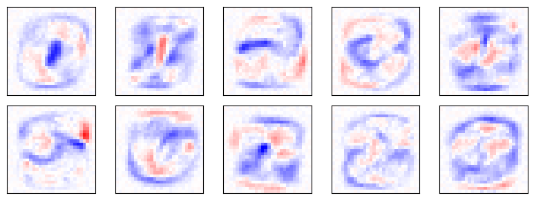
Each panel is one row of $W$ , reshaped back into a $28 \times 28$ image: the template for digits 0 to 4 (top) and 5 to 9 (bottom). The colormap is centered so that white is a weight of zero. Red pixels are positive weights, where ink raises that digit’s score; blue pixels are negative weights, where ink lowers it.

These aren’t pictures of digits. Much of what the model learned is negative evidence. The 0 template’s strongest feature is the blue blob in the middle, since ink in the center means it’s not a zero, with only a faint red ring around it. The 1 template is a red vertical stroke flanked by blue, where a wider digit would put ink. The model didn’t learn what each digit looks like so much as what distinguishes it from the other nine.

model.fc.bias

Summary¶

A linear classifier is template matching. Each class score is the dot product of the image with one learned 784-pixel template, plus a bias. That’s the same idea as the digit recognition through averages exercise, except that here training chooses the templates.
Learned templates encode differences. Because training is rewarded only for picking the right class, the templates aren’t pictures of digits. As the weight maps show, much of what they hold is negative evidence: where ink rules a digit out.
One template per class is the limit. The model reaches about 92% and stops improving. A single template can’t cover all the ways people write a digit, and each weight is tied to a fixed pixel position, so the same digit shifted by a couple of pixels looks like a different pattern.
Next: local features. A convolutional network instead learns small filters that are applied at every position of the image, and combines their responses in later layers. It gets to about 99%.