Numpy Tutorial

stough, 202-

Numpy is a powerful toolkit for the handling of large N-dimensional arrays or matrices, conveniently wrapped in Python. Given the relative inefficiencies of handling large lists of numbers in native Python, Numpy ndarrays have become the backbone of scientific computation in Python. In this notebook we’ll first show some time comparisons between ndarray and Python list basic functions, then explore some of the very useful Numpy methods.

This is a highly stripped-down introduction. The intent is to learn much of what we need along the way, as we find uses for some of Numpy’s functionality. However, See Numpy’s own quickstart tutorial for a more complete introduction.

1. Speed Comparisons

2. Numpy Essentials

   1. Indexing operations

   2. Multi-dimensional ndarrays

Imports¶

As a matter of clarity, I usually try to include all needed imports at the beginning of any notebook or script. Of note here:

• The %matplotlib inline magic command starts up the matplotlib visualization package. You can read more in the Matplotlib tutorial.

• I import numpy and then set the random number generator’s seed. This sets the state of numpy’s RNG so that every run through this notebook will be identical. While I send the seed method a constant, you could also send the current time or else nothing, and a more “random” experience will follow.

Speed Comparisons¶

We know Python lists as a really easy-to-use dynamic list implementation that includes powerful object-oriented and functional interactions, where elements of a list can be of any type. This flexibility of the list type is accomplished through the use of pointers in a way that is hidden from the programmer--under the hood--but that negatively impacts performance. Numpy on the other hand constrains all elements of an ndarray to be of the same type; under the hood, numpy arrays can be stored in contiguous memory with constant access time.

A tremendous speedup results from executing numpy’s compiled library code on contiguous memory, versus Python’s native implementations that require dealing with pointer indirection and the potential resulting scattered memory access (which impacts cache performance for example).

To demonstrate this, we’ll make a Python list of random integers using numpy’s randint, a (uniformly distributed) random number generator. We’ll also make a numpy ndarray copy of that list. This copy will be in memory that is independent of the list, which we are just copying the values from.

Then we can test certain functionality on the list and ndarray collections separately, using IPython’s timeit magic command..

The expression we’re timing is min(lyst), which is the Python function to return the minimum of any iterable of comparable types in Python. The default output of timeit tells us with some degree of certainty how much wall time calculating min(lyst) is likely to take, probably in units of microseconds $\mu s$. timeit computes this by taking several runs (default 7) and each time executing the expression potentially thousands of times to get to some precision in the measurement.

You should notice a significant speedup in the np.min() result over the Python min() result. On my machine I observe ~3x speedup on a list of length 1000 (1K). In that there is always some baseline overhead cost due to the Python interpreter (as opposed to compiled library calls), you may notice that the speedup improves the larger the list size is made to be. I observed a ~12x speedup on a list size of 10K, and a 15-20x speedup beyond 100K.

One significant caveat here is that there is a big precision reduction: the integer primitive in Python is for arbitrary magnitude integral values and requires 28 bytes, while the implicitly determined np.int64 requires only 8 bytes with a more limited magnitude range. In conjunction with the direct packing (instead of pointer packing) in memory, the ndarray variable np_lyst requires much less memory than the Python variable lyst, and likely engenders much better cache coherence (read: average memory access time). Read more about it here or here. Additionally it is possible to write your own efficient C code implementations that can be called from Python: read (much) more here.

Computing the minimum of a collection is a straightforward linear complexity problem, $O(n)$. We’ll now try another example, this time of sorting a list/ndarray, which you’ll remember generally has complexity $O(n\log{}n)$.

Both the sorted() and np.sort() methods are functions in the sense that they do not modify the argument collection (whether list or ndarray), but rather return a sorted copy of that collection. Alternative object-oriented in-place sort and ndarray.sort methods are also available. However, for the purposes of timing, sorting an already sorted list is pretty uninteresting. In the sorting experiment above, I observed ~2-4x speedup using the Numpy equivalent on list size 1K.

The final timing examples above show the efficiency of Python list comprehensions and the equivalent numpy expression. The above list comprehensions (or list(map(...) create a new list object where every element of the original list has been scaled by a constant. Such Pythonic expressions execute in interpreted bytecode, which can be quite a bit slower than comparative compiled C. Using smart operator overloading, the creators of Numpy encoded equivalent functionality that executes almost entirely in C, resulting in significant speedup (e.g., ~70x on list size 10K in my observations). We can actually observe this efficiency indirectly just in the amount of bytecode involved in the competing approaches, using Python’s disassembler module.

As an aside, ndarrays are static in that they cannot change size easily (without $O(n)$ cost). While this is a deficiency relative to Python’s dynamic list implementation (with ammortized $O(1)$ cost to append), this is not much of a problem usually.

Across computational workflows much more complicated than the above simple experiments demonstrate, people have found Numpy to be up to 100 times faster than native Python. To be clear, ndarrays cannot easily replace all Python lists in our lives: we are after all programming in Python! But in computationally intensive endeavors like image processing, where dealing with millions of pixels is an every second kind of thing, we will have to leverage Numpy’s massive speedups.

Numpy Essentials¶

As demonstrated above, Numpy often provides vastly superior performance for computationally intensive tasks on collections of data. Additionally, it also provides great new functionality that becomes quite useful in scientific computing contexts: index-related operations, dimension swapping, conditional filtering, etc.. In this section we’ll explore some of this functionality. We’ll also show similar Python list functionality in case that helps understanding. I’ll often refer to the official Numpy documentation.

Let’s start by making a small ndarray with random integer values for pedagogical purposes. All of the same examples could be easily extended to floating point or much larger arrays.

Indexing Ops¶

We’ll start with index-related operations. It is often advantageous to reorder collections (for example sorting) in a way that is reversible. To do this we need to record where each element came from. It’s easy enough to get an index along with the associated element using enumerate.

Then, let’s try finding the index of the minimum.

As you can see, ndarray’s argmin or equivalent numpy.argmin() methods can replace a bit of Python code. See also ndarray.argmax. Also note there are often equivalent functional numpy and object-oriented ndarray methods, as in np.argmin(np_lyst) and np_lyst.argmin() above.

We are often also interested in where some condition is true, as in ‘is this element greater than 50’ or ‘is this part of an image sky.’ We can use numpy.where() to get at that kind of information:

In the above cells, I print out the elements of the ndarray, then the elements of a conditional array np_lyst > 50, then the output of the where() call. I also pretty-print the arrays for a little more clarity, which you can read a lot more about here.

As you can see, when where() is sent an array, it will return an array of indices where non-zero (or non-False) elements can be found. You can actually see it’s returning a tuple, which becomes relevant for multidimensional arrays--but we’ll leave that for when it’s actually relevant. A call to ndarray.nonzero on the conditional array itself is equivalent in this case:

However where is quite a bit more powerful. We can use where to sample from two sources based on the condition argument. In the below, whenever the condition > 50 is True in np_lyst, we sample the element directly, and otherwise the square root of the element is used.

Multi-dimensional ndarrays¶

Every ndarray object represents a multi-dimensional matrix of data. The hardest part about dealing with such large structured collections of data is always to keep in mind any particular ndarrays shape, dimensionality, and type of data, often along with the range of the data inside. Fortuitously, this is easily accessible in Numpy arrays through attributes and simple method calls.

Let’s start simple by instantiating a couple of 2D ndarrays.

You can see above that a and b are 4x6 matrices. In order to get at all of the details I mention above, let’s make a reusable function

The arr_info function here accesses and returns the arr argument’s shape and dtype attributes and calls on the min and max methods to give us a snapshot of the content. The dimensionality of arr is the length of the shape tuple returned (or also a.ndim would work). This arr_info function is so useful, we’ll source it out to common utilities.

There are a number of things to note about the above cell and its output:

• a/b means element-wise division. In fact all arithmetic ops between ndarray objects are element-wise.

• In order for element-wise to make sense, both operands (a and b) must be broadcastable to the same shape. For example, a/4 would work because 4 can be broadcast to 4x6 (copies of the number 4).

• The result of a/b (and other such ops) is in fact a new ndarray object, which is then assigned the variable name c.

• The result of integer division is floating point (see dtype('float64') above).

• This arr_info function has been abstracted the matrix_utils module for use throughout this book.

We can slice and index an ndarray matrix in the same way we would a Python list of lists. Here, we’ll make a 3x4 matrix and view some slices of it.

As seen above, we can slice an ndarray pretty easily (at least compared to the list equivalent).

• As with Python slicing, :k means up to but not including index k, while j: means starting at index j and continuing through the end.

• : and ... happen to mean the same in the above cells only because a is 2D. For a matrix of higher dimensionality, a[...,:2] would mean a[:,:,:2] or a[:,:,:,:2] or so on. That is, for all dimensions iterate over all elements until the last dimension involving a different slice.

Let’s up the dimensionality to 3. We’ll reshape the 12 elements of a to be 2x2x3 instead of 3x4.

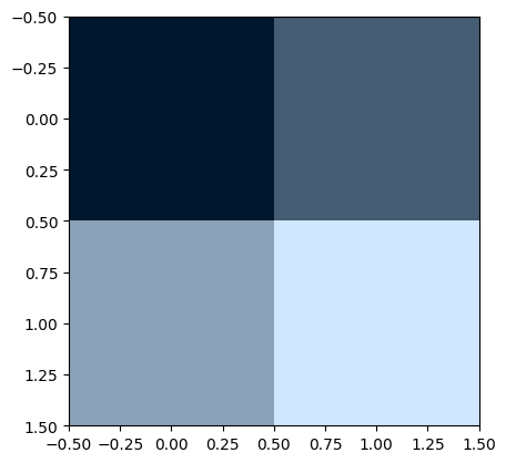
The reshaping we did here could for example represent a 2 pixel by 2 pixel image with 3 ‘color channels.’ If the three color channels represent the amount of red, green, and blue, then each pixel would have a bluish hue since blue > green > red in the last or ‘color’ dimension. But here we’re getting ahead of ourselves.

We can also transpose dimensions or flip the order of elements within one dimension.

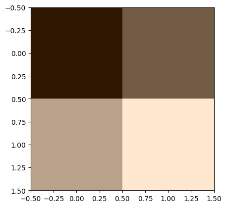
When we np.flip() axis 2 (the last of the 2x2x3 matrix) of a, we make red > green > blue. As a result each pixel has a beige hue. But again, we’re getting ahead of ourselves...

This has been a very brief introduction to some Numpy and ndarray functionality and interaction. We will pick up more as we need it; as in the malaphor, “We’ll burn that bridge when we get to it.” Again, see Numpy’s own quickstart tutorial for a more complete and abstract introduction.