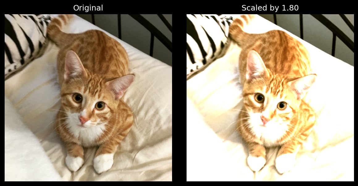
Interactive Visualizations Tutorial - imageprocessing-awesome

Preview: Interactive Visualizations Tutorial

stough, 202-

This is a very brief introduction to interactive visualization or animation in ipympl. We’ve seen in the matplotlib tutorial that ipympl provides for some interaction, like zooming and dragging. But often we want to change the actual content of the plots based on the interaction. For this example I’ll show the commented code, the demonstration, and then a short review. We’ll introduce even more complicated examples only as needed. There are numerous resources on this topic, and many examples may not quite work given the particular library versions you’re working with: setup can be pretty brittle.

Imports¶

%matplotlib inline
import matplotlib.pyplot as plt
import scipy.ndimage as ndimage
import numpy as np

from scipy.ndimage import correlate
from skimage.filters import *

from ipywidgets import VBox, FloatSlider, AppLayout

plt.style.use('dark_background')

Slider Interaction¶

This example is one we’ll rip directly from ipympl (specifically this one)

pass  # (static) plt.ioff()

# Create a slide object
slider = FloatSlider(
    orientation='horizontal',
    description='Factor:',
    value=1.0,
    min=0.02,
    max=2.0
)

slider.layout.margin = '0px 30% 0px 30%'
slider.layout.width = '40%'


# Plot and title the initial display. 
fig = plt.figure()
fig.canvas.header_visible = False
pass  # (static) fig.canvas.layout.min_height = '400px'
plt.title('Plotting: y=sin({} * x)'.format(slider.value))

x = np.linspace(0, 20, 500)

lines = plt.plot(x, np.sin(slider.value * x))


# A function that will be called whenever the slider changes.
def update_lines(change):
    # plt.title('Plotting: y=sin({} * x)'.format(slider.value))
    plt.title(f'Plotting: y=sin({slider.value: .3f} * x)')
    lines[0].set_data(x, np.sin(change.new * x))
    fig.canvas.draw()
    fig.canvas.flush_events()

# Connecting the slider object to the update function above.
# This is event-handling.
slider.observe(update_lines, names='value')

# Creates an application interface with the various 
# pieces we already instantiated inside of it. 
pass  # (static) AppLayout(
pass  # (static)     center=fig.canvas,
pass  # (static)     footer=slider,
pass  # (static)     pane_heights=[0, 6, 1]
pass  # (static) )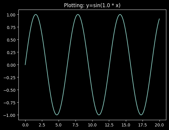

The key pieces in the above example are pretty straightforward once you get the hang of it. We’re basically producing different constituent objects, tying them together, so that data from one can be passed to another, then packing these objects together in an app and displaying the app.

slider = FloatSlider...: a horizontal slider is instantiated with some range and explicit initial value. Many other parameters (like step size) default, but you may find them useful. Read more here.
Some plot is produced: Various distracting layout info is there, but keys are the creation of a (current) figure with plt.figure(), plt.title to produce a title, and plt.plot to draw a line plot given x,y. Important here is that the return value of the plot function is actually a list of Line2D objects, a complicated under-the-hood bit of matplotlib (there’s actually only the one sin curve line object, it’s just inside a list). Notice also that we use slider.value in that first plot. slider is an object and its current positional value is in the property value.
def update_lines(change)...: This is the function that will be called every time the user moves the slider. Key pieces in the function are that we re-title the plot (so that the title can be dynamic) and we set/change the data inside the Line2D object we originally plotted through the set_data call.
slider.observe(update_lines, names='value'): When the value property of the slider object is updated (click-and-drag by the user for example), then update_lines will be called with a parameter we’ve named change. This is a weird object, but suffice to say the expression change.new is the value of the slider inside the update_lines function. We can also directly use the expression slider.value since that object is defined within the same cell. I do both just to show.
AppLayout...: Lastly we put the plot (with title) and slider objects together in an AppLayout object. We only have two things to stuff into the app, the figure we plotted, and the slider object.

Whew, that’s it! As you probably see by now, it is insanely useful to start with ripped code whenever you’re hoping to accomplish something interesting in these interactive displays. I will be providing such code demos throughout this book.

Interactive Image Display¶

The sine example above updates a line. Throughout this book though, we’ll mostly be updating images: changing some parameter of a transform with a slider and watching the result change. The pattern is nearly identical, with a couple of small differences you’ll see again and again:

the figure and slider are stacked with a simple VBox rather than an AppLayout;
instead of set_data on a Line2D, we call set_data on the AxesImage that imshow returns;
we turn interactive mode off (plt.ioff()) before building the figure, so the figure only appears inside our VBox and not a second time on its own.

Let’s brighten (or darken) an image by scaling its intensities.

I = plt.imread('../dip_pics/cat_small.png')[..., :3] # drop the alpha channel; floats in [0,1]

pass  # (static) plt.ioff()

bright_slider = FloatSlider(
    orientation='horizontal',
    description='Scale:',
    value=1.0,
    min=0.0,
    max=3.0,
    step=0.05
)

fig, ax = plt.subplots(1, 2, figsize=(8,4), num='Interactive brightness')
fig.canvas.header_visible = False

ax[0].imshow(I)
ax[0].set_title('Original')

# Keep the AxesImage returned by imshow: this is what we'll update.
rdisp = ax[1].imshow(I)
rtext = ax[1].set_title(f'Scaled by {bright_slider.value:.2f}')

for a in ax:
    a.set_axis_off()

def update_image(change):
    # Scale, then clip back into the valid [0,1] float range for display.
    rdisp.set_data(np.clip(change.new * I, 0, 1))
    rtext.set_text(f'Scaled by {change.new:.2f}')
    fig.canvas.draw()
    fig.canvas.flush_events()

bright_slider.observe(update_image, names='value')

plt.tight_layout()

pass  # (static) VBox([bright_slider, fig.canvas])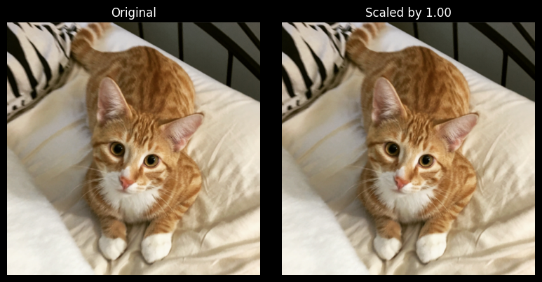

Compare this to the sine example and you’ll see the same three moves: make the widget, make the plot while holding on to the artist you want to change (rdisp), and connect the two through an update function and observe.

A couple of details matter for images:

We np.clip the scaled image. A float RGB image in matplotlib must be in $[0,1]$ . Values outside that range get clipped anyway, with a warning, so it’s better to do it ourselves. (We’ll look at exactly this kind of transfer function in the enhancement chapter.)
Notice what happens as you drag the slider past 1: brighter, sure, but more and more of the image saturates to white, and that detail is gone for good. Scaling below 1 darkens without losing anything, at least until we quantize back to integers.
rdisp.set_data only replaces the pixel values. The color limits imshow chose the first time stay fixed. That’s what we want for RGB images, but for a single-channel image shown with a colormap you might also need rdisp.set_clim(...).

Once you’re done with an interactive figure, it’s good practice to close it and turn interactive mode back on, so it doesn’t reappear when later cells draw:

plt.close('Interactive brightness')
plt.ion()

<contextlib.ExitStack at 0x7fe3e0265d30>