stough 202-
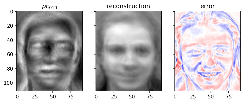
Let’s reconstruct a face according to the pca trained on the ORL faces dataset.
In Face Space and Component Spans we used PCA to look at faces. Here we use it to rebuild one, adding back one principal component at a time, just like the partial reconstructions of a pixel-art image with the Haar basis. The PCA basis of faces is the KLT basis (see view_basis_blocks) for whole face images.
%matplotlib inline
import matplotlib.pyplot as plt
import numpy as np
from matplotlib.offsetbox import (OffsetImage,
                                  AnnotationBbox)
import matplotlib.animation as animation
from sklearn.decomposition import PCA
from skimage.color import rgb2gray

from torchvision import transforms
from torchvision.datasets import ImageFolder

# For importing from alternative directory sources
import sys
sys.path.insert(0, '../dip_utils')
from data_paths import orl_root

NUMPCA = 400
IMAGE = None
# IMAGE = '../dip_pics/josh_thumbnail.png' # must be a 112x92 face image

imshape = (112, 92)
orl_faces = ImageFolder(orl_root(),
transform=transforms.Compose([
transforms.Grayscale(),
transforms.ToTensor(),
transforms.Lambda(lambda x: np.array(x).ravel())
]))
allfaces = np.stack([orl_faces[i][0] for i in range(len(orl_faces))])# Now get NUMPCA most important 10304-d directions in the space of faces.
pca = PCA(n_components=NUMPCA)
Xp = pca.fit_transform(allfaces) # Xp is 400 x 10, the 10-pca dimensional projections of each image.
print('Explained variation per principal component: {}...'.format(pca.explained_variance_ratio_[:20]))
print(f'Total variance explained in {NUMPCA} dimensions: {np.sum(pca.explained_variance_ratio_)}')np.sum(pca.explained_variance_ratio_[:20])This time we ask for all 400 components (we have 400 faces, so that’s as many as there can be). The first 20 alone explain about 70% of the variance.
Now we’ll reconstruct some image.
if IMAGE is None:
    which = np.random.choice(len(allfaces))
    I = np.reshape(allfaces[which,:], imshape).copy()
    coeff = Xp[which, :].squeeze()
else:
    I = rgb2gray(plt.imread(IMAGE))
    coeff = pca.transform(I.ravel()[None,:]).squeeze()
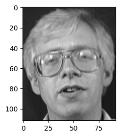
We pick a random face from the dataset and get its 400 PCA coefficients, the weights such that . Alternatively, set IMAGE at the top to your own grayscale face photo, which will be projected onto the same components.
f, ax = plt.subplots(1,1,figsize=(3,3))
ax.imshow(I, cmap='gray')
plt.show()
Expected output (what the cell above should show, if you can’t run it)
# We need to include the mean as though it is one of the dimensions
# that can be added...
# And let's also reorder the pcas

# In order of absolute magnitude
# inorder = np.arange(0, len(coeff))
inorder = np.argsort(np.abs(coeff))[::-1]

pcas = np.concatenate([pca.mean_[None,:], pca.components_[inorder]], axis=0)
coeff = np.array([1] + list(coeff[inorder]))
Two bookkeeping tricks. First, we put the mean face at the front of the list of “components”, with a coefficient of 1, so reconstruction is just a weighted sum: coeff[:k+1] @ pcas[:k+1]. Second, we add the components in order of the magnitude of this face’s coefficients, rather than in the usual order of explained variance. That way each step adds the component that matters most for this particular face, which is the same greedy choice as keeping the largest transform coefficients in compression.
def reconstruct(ind):
    global pcas, coeff, imshape
    return np.reshape(np.matmul(coeff[:ind+1], pcas[:ind+1]), imshape)
from ipywidgets import VBox, IntSlider
pass # (static) plt.ioff()
plt.clf()
slider = IntSlider(
orientation='horizontal',
value=0,
min=0,
max=NUMPCA,
description='$c_i$'
)
curi = 0
Ir = np.reshape(pca.mean_, imshape)
AvgFace = Ir.copy()
# Figure display and artists.
fig_args = {'num':' ', 'frameon':True, 'sharex':True, 'sharey':True}
fig, ax = plt.subplots(1,3, figsize=(8,3), **fig_args)
ldisp = ax[0].imshow(Ir, cmap='gray')
ltext = ax[0].set_title('mean')
mdisp = ax[1].imshow(Ir, cmap='gray')
ax[1].set_title('reconstruction')
rdisp = ax[2].imshow(I-Ir, cmap='bwr')
ax[2].set_title('error');
# updatefig function
def update_image(change):
global curi, inorder, pcas, Ir, ldisp, I, ltext, mdisp, rdisp, imshape
# See where change.new is versus curi.
# Then update the reconstruction
# This was pointless! Both for the difficulty of coding
# and for the accumulation of floating point error.
# newi = change.new
# diff = newi - curi
# if diff > 0:
# while curi != newi:
# curi += 1
# Ir = Ir + np.reshape(coeff[curi]*pcas[curi], imshape)
# elif diff < 0:
# while curi != newi:
# curi -= 1
# Ir = Ir - np.reshape(coeff[curi]*pcas[curi], imshape)
curi = change.new
pc = np.reshape(pcas[curi], imshape)
ldisp.set_array(pc)
ldisp.set_clim(pc.min(), pc.max())
# Tried, but failed, to add tex math in an f-string:
# https://stackoverflow.com/questions/50209287/evaluating-variable-contain-mathematical-expression-in-f-strings
# ltext.set_text(f'$pc_{{curi}}$')
# ltext.set_text(r'$pc_{:03d}$'.format(curi)) # only the first digit is subscript
# This works because the old %format style does not conflict with the use of {} in math tex.
ltext.set_text('$pc_{%03d}$' % curi)
Ir = reconstruct(curi)
mdisp.set_array(Ir)
mdisp.set_clim(Ir.min(), Ir.max())
rdisp.set_array(I-Ir)
fig.canvas.draw()
fig.canvas.flush_events()
slider.observe(update_image, names='value')
pass # (static) VBox([slider, fig.canvas])Expected output (what the cell above shows after slider.value = 10)
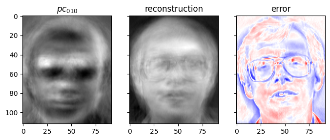
Drag the slider. The left panel shows the component just added, the middle the reconstruction so far, and the right the remaining error (red and blue for positive and negative). Starting from the mean face, the reconstruction becomes recognizable as the right person within a few dozen components, and the error image fades toward white as the slider goes up.
Because this face was one of the 400 PCA was fit to, using all 400 components reconstructs it exactly. Try setting IMAGE to a face that wasn’t in the training set: the reconstruction then levels off with some error that never goes away. That leftover is the part of the new face that lies outside the “face space” spanned by these 400 faces. How far a new image is from face space is itself a useful number. It can tell you whether an image is a face at all.