Intro to Principal Components Analysis - imageprocessing-awesome

stough 202-

Preview: Intro to Principal Components Analysis

A brief look at principal components on real data. If you haven’t yet, start with PCA in 2D, where we can see everything PCA does.

The Iris dataset example we’re using here
Khan academy videos on Linear Algebra background.
Kind of a neat walkthrough of this same Iris dataset.

The classic Iris dataset has 150 flowers from three species of iris, with four measurements of each: sepal length, sepal width, petal length, and petal width (in cm). So each flower is a point in 4D, which we can’t look at directly.

%matplotlib inline
import matplotlib.pyplot as plt
import numpy as np
from mpl_toolkits.mplot3d import Axes3D
from sklearn import datasets
from sklearn.decomposition import PCA

# import some data to play with
iris = datasets.load_iris()

X = iris.data
y = iris.target

x_min, x_max = X[:, 0].min() - .5, X[:, 0].max() + .5
y_min, y_max = X[:, 1].min() - .5, X[:, 1].max() + .5

f, ax = plt.subplots(1,1, figsize=(5,5))

# Plot the training points
ax.scatter(X[:, 0], X[:, 1], c=y, cmap=plt.cm.Set1,
            edgecolor='k')
plt.xlabel(iris.feature_names[0])
plt.ylabel(iris.feature_names[1])

plt.xlim(x_min, x_max)
plt.ylim(y_min, y_max)
plt.xticks(())
plt.yticks(());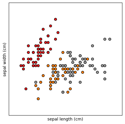

Any single pair of the four measurements is only a partial view. Here, with sepal length and width, one species (red) separates nicely from the others, but the other two overlap a lot. Which 2D or 3D view of the 4D data shows the most? PCA’s answer: the view along the directions of greatest variance.

# To getter a better understanding of interaction of the dimensions
# plot the first three PCA dimensions
fig = plt.figure(figsize=(5,5))
# ax = Axes3D(fig)# , elev=-150, azim=110)
ax = fig.add_subplot(111, projection='3d')

pca = PCA(n_components=3)
X_reduced = pca.fit_transform(iris.data)
ax.scatter(X_reduced[:, 0], X_reduced[:, 1], X_reduced[:, 2], c=y,
           cmap=plt.cm.Set1, edgecolor='k', s=40)
ax.set_title("First three PCA directions")
ax.set_xlabel("1st eigenvector")
ax.set_xticklabels([])
ax.set_ylabel("2nd eigenvector")
ax.set_yticklabels([])
ax.set_zlabel("3rd eigenvector")
ax.set_zticklabels([])
# plt.show()

[Text(-1.0, 0, ''),
 Text(-0.8, 0, ''),
 Text(-0.6, 0, ''),
 Text(-0.3999999999999999, 0, ''),
 Text(-0.19999999999999996, 0, ''),
 Text(0.0, 0, ''),
 Text(0.20000000000000018, 0, ''),
 Text(0.40000000000000013, 0, ''),
 Text(0.6000000000000001, 0, ''),
 Text(0.8, 0, ''),
 Text(1.0, 0, '')]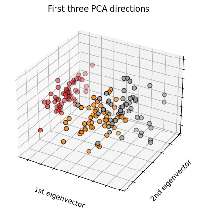

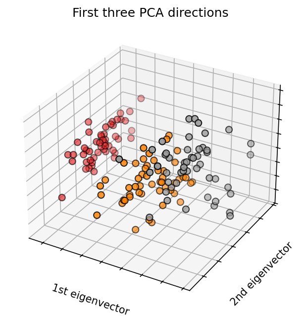
Rotate this plot around. The three species now spread out much more cleanly, mostly along the first principal direction. We haven’t told PCA anything about species: it only looked for the directions of greatest variance, and it happens that the biggest differences among these flowers are the differences between species. That’s common, and it’s why PCA is so often the first thing to try on new data. It isn’t guaranteed, though, since the direction that varies most need not be the one you care about.

Let’s explore the PCA itself.¶

# The first couple of principal components already account for a lot 
# of the variance in the data.
import numpy as np
print('The first two pca dims represent '\
      f'{sum(np.var(X_reduced[:,:2], axis=0)) / sum(np.var(X, axis=0)):.3f} '
      'fraction of the original data.')

The first two pca dims represent 0.978 fraction of the original data.

Two of four dimensions capture almost 98% of the total variance. The other two directions hold barely 2%, so the 4D data is very nearly flat.

The linear combinations required¶

of the original 4 components, to construct each principal component.

See PCA reference.

# What linear combinations does the PCA discover.
pca.components_

array([[ 0.36138659, -0.08452251,  0.85667061,  0.3582892 ],
       [ 0.65658877,  0.73016143, -0.17337266, -0.07548102],
       [-0.58202985,  0.59791083,  0.07623608,  0.54583143]])

Each row is a principal component, a unit vector in the original 4D measurement space. The first row tells us that PC1 is about $0.36\times$ sepal length $- 0.08\times$ sepal width $+ 0.86\times$ petal length $+ 0.36\times$ petal width. It’s dominated by petal length, with petal width and sepal length chipping in, so roughly “overall flower size, especially the petals”. (One caveat: we didn’t standardize the measurements, so features with larger spreads, like petal length, naturally get more weight.)

# Notice that they're orthogonal, just like we said before, 
# with block transform encoding.
np.dot(pca.components_[0,:], pca.components_[1,:])

np.float64(-2.3592239273284576e-16)

np.sum(pca.components_**2, axis=1)

array([1., 1., 1.])

pca.explained_variance_ratio_

array([0.92461872, 0.05306648, 0.01710261])

The explained variance ratios: the first component alone holds about 92% of the variance, which is why the species already separate along a single axis.