Spanning PCA dimensions.

stough 202-

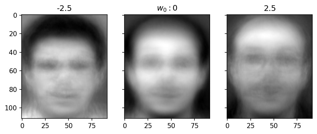
In this visualization, we sort all the faces by their coefficient in the 0th (most important) pca dimension. Then we just loop over them.

Second, we also show the abstract ‘face’ $\pm 2\sigma$ in the 0th pc.

The goal is to understand what a principal component means. A component is a direction in the space of faces. Walking along it (keeping every other coefficient fixed at the average) should change faces in one consistent way. We’ll see this two ways: with real faces ordered by their coefficient, and with synthetic faces built as the mean plus a multiple of the component. See Face Space for the setup.

%matplotlib inline
import matplotlib.pyplot as plt
import numpy as np
from matplotlib.offsetbox import (OffsetImage,
                                  AnnotationBbox)
import matplotlib.animation as animation
from sklearn.decomposition import PCA

from torchvision import transforms
from torchvision.datasets import ImageFolder

# For importing from alternative directory sources
import sys  
sys.path.insert(0, '../dip_utils')
from data_paths import orl_root
NUMFACES = 20 # Number of random faces to display in the first scatterplot
NUMSUBJECTS = 3 # Number of subjects to display in the subject-specific scatter

imshape = (112, 92)

orl_faces = ImageFolder(orl_root(), 
                       transform=transforms.Compose([
                           transforms.Grayscale(),
                           transforms.ToTensor(),
                           transforms.Lambda(lambda x: np.array(x).ravel())
                       ]))

faces = np.stack([orl_faces[i][0] 
                  for i in np.random.choice(len(orl_faces), NUMFACES)])
allfaces = np.stack([orl_faces[i][0] for i in range(len(orl_faces))])

# Now get 10 most important 10304-d directions in the space of faces.
pca = PCA(n_components=10)
Xp = pca.fit_transform(allfaces) # Xp is 400 x 10, the 10-pca dimensional projections of each image.
print('Explained variation per principal component: {}'.format(pca.explained_variance_ratio_))

# First, show the average and first two pca directions

f, ax = plt.subplots(1,3, figsize=(9, 3), sharey=True, sharex=True)
f.suptitle('Average Face and Two Principal Components')
ax[0].imshow(np.reshape(allfaces.mean(axis=0), imshape), cmap='gray')
ax[0].set_title('Average Face')

# pca.components_ is 10 x 10304 here, representing the most meaningful
# directions in the 10304-d space of face images.
ax[1].imshow(np.reshape(pca.components_[0,:], imshape), cmap='gray')
ax[1].set_title('PCA 1')

ax[2].imshow(np.reshape(pca.components_[1,:], imshape), cmap='gray')
ax[2].set_title('PCA 2');

Faces sorted along the first principal component.¶

# Now, animate from one extreme to the other in the first pca direction.

inorder = np.argsort(Xp[:,0]) # Sort on the first pca dimension.

f2, ax2 = plt.subplots(1, 3, figsize = (9, 3), sharex=True, sharey=True)
f2.suptitle('Faces Sorted According to PCA 1 Score')

ax2[0].imshow(np.reshape(allfaces[inorder[0]], imshape), cmap='gray')
ax2[2].imshow(np.reshape(allfaces[inorder[-1]], imshape), cmap='gray')

cI = ax2[1].imshow(np.reshape(allfaces[inorder[0]], imshape),
                   cmap='gray', animated=True)

whicharg = 0

cIText = ax2[1].text(10, 105,
                     '%d, %7.2f' % (whicharg, Xp[inorder[whicharg],0]),
                     fontsize=10, color='k')



# Needs to update the array data and the texts, then
# return the artists. see:
# https://matplotlib.org/api/_as_gen/matplotlib.animation.FuncAnimation.html
#
def updateFig(*args):
    global faces, whicharg, inorder, Xp

    cI.set_array(np.reshape(allfaces[inorder[whicharg]], imshape))

    cIText.set_text('%d, %7.2f' % (whicharg, Xp[inorder[whicharg], 0]))

    whicharg += 1
    if whicharg == len(inorder):
        whicharg = 0

    return cI, cIText,

ani = animation.FuncAnimation(f2, updateFig, interval=300, blit=True, repeat=False)

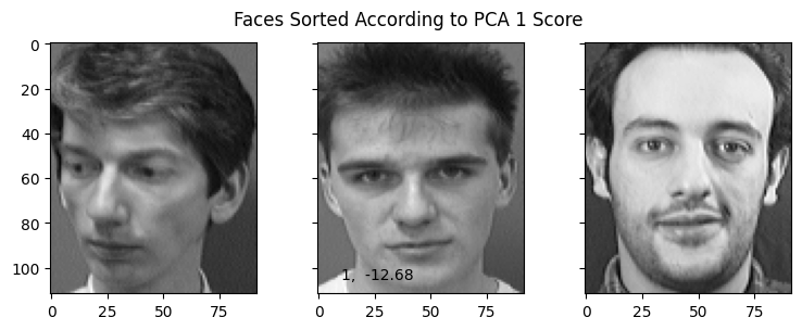
The left and right images are the faces with the lowest and highest first PCA coefficient, and the middle animates through all 400 faces in order of that coefficient, which is printed at the bottom. As it plays, notice what changes steadily from one end to the other. (Individual faces vary in many other ways at the same time, so look for the overall trend.)

$\pm 2\sigma$ on $PC_0$ ¶

# We're only going to change one image, but I want to see the two end points 
varmax = 2.5
sigmas = np.sqrt(pca.explained_variance_)
face_neg = np.reshape(pca.mean_ - varmax*sigmas[0]*pca.components_[0,:], imshape)
face_pos = np.reshape(pca.mean_ + varmax*sigmas[0]*pca.components_[0,:], imshape)

def makeinterp(coeff):
    global pca, sigmas, imshape
    return np.reshape(pca.mean_ + coeff*sigmas[0]*pca.components_[0,:], 
                      imshape)

makeinterp builds a synthetic face: the mean face plus coeff standard deviations along the first component, $\boldsymbol{\mu} + w_0\,\sigma_0\,\mathbf{v}_0$ . Since nearly all real faces have coefficients within about $\pm 2.5\sigma$ , the slider’s range spans the realistic extremes. The two end faces are no particular person. They show what “more” or “less” of this component looks like, with everything else held at average.

from ipywidgets import VBox, FloatSlider

pass  # (static) plt.ioff()
plt.clf()

slider = FloatSlider(
    orientation='horizontal',
    value=0.0,
    min=-varmax,
    max=varmax,
    description='$w_0$'
)


fig_args = {'num':' ', 'frameon':True, 'sharex':True, 'sharey':True}
fig, ax = plt.subplots(1,3, figsize=(8,3), **fig_args)


Ic = makeinterp(0);

# display artists I'll update
ldisp = ax[0].imshow(face_neg, cmap='gray')
ax[0].set_title(f'{-varmax}')

mdisp = ax[1].imshow(Ic, cmap='gray')

rdisp = ax[2].imshow(face_pos, cmap='gray')
ax[2].set_title(f'{varmax}')

mtext = ax[1].set_title(f'$w_0: 0$')


# updatefig function
def update_image(change):
    global Ic, mdisp
    Ic = makeinterp(change.new)
    mdisp.set_array(Ic)
    mdisp.set_clim(Ic.min(), Ic.max())
    mtext.set_text(f'$w_0: ${change.new}')  # '{}*LaPlace'.format(change.new))
    fig.canvas.draw()
    fig.canvas.flush_events()

slider.observe(update_image, names='value')

pass  # (static) VBox([slider, fig.canvas])

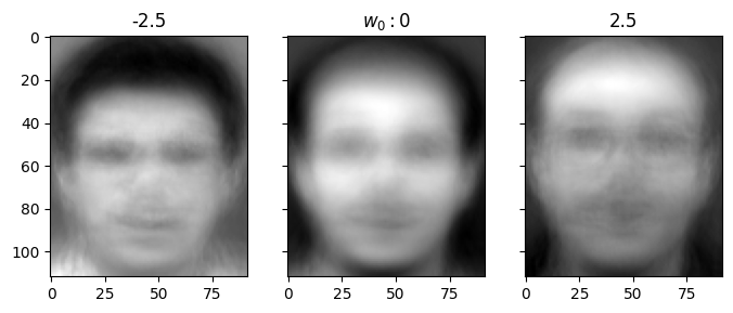
Slide back and forth. For the ORL faces, the first component mostly changes how bright the face is against its background, more a matter of lighting and exposure than of who is in the photo. That’s typical: the largest variations in a set of photos are often about the photography rather than the subject, which is one reason eigenface recognizers often skip the first few components. Try changing [0] to [1] or [2] in makeinterp and the face definitions, to explore the next components. You’ll find mixtures of lighting direction, hairline, glasses, and head position. Unlike the measurements of the Iris flowers, face components rarely have clean names.

Faces sorted along the first principal component.¶

±2σ\pm 2\sigma±2σ on PC0PC_0PC0​¶

$\pm 2\sigma$ on $PC_0$ ¶