Playing around with PCA on MNIST data. - imageprocessing-awesome

stough 202-

Preview: Playing around with PCA on MNIST data.

We’re going look at Principal Component Analysis and the MNIST data today, and an analogy with some of the block transform and image compression stuff we’ve done before.

MNIST is 70,000 small ( $28 \times 28$ ) grayscale images of handwritten digits, which we’ll use a lot in the machine learning chapter. In the block transform chapter we saw fixed bases (Haar, DCT) for representing image blocks. Here we let PCA learn a basis from 60,000 example digits, and see how few basis images it takes to represent a digit well. (If you haven’t, see PCA in 2D first.)

Import¶

A lot. We need MNIST data, PCA, and all of our block transform materials.

%matplotlib inline
import matplotlib.pyplot as plt
import numpy as np

# For the MNIST data
from torchvision import datasets, transforms
from torchvision.utils import make_grid

# For PCA 
from sklearn.decomposition import PCA

from skimage.util import montage

# For importing some of our own utility codes.
import sys  
sys.path.insert(0, '../dip_utils')

from data_paths import mnist_root
from matrix_utils import (arr_info,
                          make_linmap)
from vis_utils import (vis_rgb_cube,
                       vis_hists,
                       vis_pair)

from wavelet_utils import (make_haar_matrix,
                           make_random_basis,
                           make_klt_basis,
                           make_dct_matrix,
                           make_standard_matrix,
                           vis_blocks)

Loading and Formatting the MNIST Data¶

# Thank you: https://www.aiworkbox.com/lessons/load-mnist-dataset-from-pytorch-torchvision
# https://pytorch.org/vision/stable/datasets.html
mnist_trainset = datasets.MNIST(root=mnist_root(), train=True, download=True, transform=None)
mnist_testset = datasets.MNIST(root=mnist_root(), train=False, download=True, transform=None)

x_train = np.stack([np.array(x).ravel() for x,_ in mnist_trainset])
x_test = np.stack([np.array(x).ravel() for x,_ in mnist_testset])
y_train = np.stack([y for _,y in mnist_trainset]).astype('long')
y_test = np.stack([y for _,y in mnist_testset]).astype('long')

# These are Nx784
x_train = x_train.astype(np.float32)/255.0
x_test = x_test.astype(np.float32)/255.0

torchvision downloads MNIST into your data folder the first time (see data_paths). We then flatten every $28 \times 28$ image into a row of 784 numbers in $[0,1]$ : x_train is $60000 \times 784$ and x_test is $10000 \times 784$ .

PCA¶

We’ll do a PCA analysis of the MNIST training set to see its power on this kind of data. Let’s use pca_spanFaces as a guide. Here each row of x_train for example represents a $28\times28$ image. PCA won’t know anything about that, and will just think we have 60K points in a 784-D space.

Here we’ll ask for the 64 most important 784-d vectors in the space of 60K mnist example images. Remember, these are directions that best explain the differences between the mnist images.

# Fit PCA to the entire training set
pca = PCA(n_components=64)  # or whatever number of components
pca.fit(x_train)

# Visualize the learned principal components as 28x28 basis images
basis_images = pca.components_.reshape(pca.n_components, 28, 28)

# Visualize them
plt.figure(figsize=(10, 10))
plt.imshow(montage(basis_images, grid_shape=(8, 8)), cmap='gray')
plt.title('PCA Basis Patterns Learned from MNIST')

These are the 64 directions of greatest variation among the digits, as $28 \times 28$ images, in order of importance (left to right, top to bottom). Gray is zero, with lighter and darker showing positive and negative weights. The first few are broad, blobby strokes, like the difference between a “0”-like ring and a “1”-like vertical bar. Later components get finer and more detailed, much like the progression from coarse to fine patterns in the Haar and DCT bases. The difference is that these patterns were learned from the data, so they look like pieces of digits.

PCA also centers the data, so every digit is represented as the mean digit plus a weighted sum of these components.

f, ax = plt.subplots(1, 2, figsize=(9,3))
ax[0].imshow(pca.mean_.reshape(28, 28), cmap='gray')
ax[0].set_title('Mean digit')
ax[0].set_axis_off()

ax[1].plot(np.arange(1, 65), np.cumsum(pca.explained_variance_ratio_), 'o-', markersize=3)
ax[1].set_xlabel('number of components')
ax[1].set_ylabel('fraction of variance explained')
ax[1].grid(alpha=.3)
plt.tight_layout()

print(f'10 components: {np.sum(pca.explained_variance_ratio_[:10]):.2f} of the variance')
print(f'64 components: {np.sum(pca.explained_variance_ratio_):.2f} of the variance')

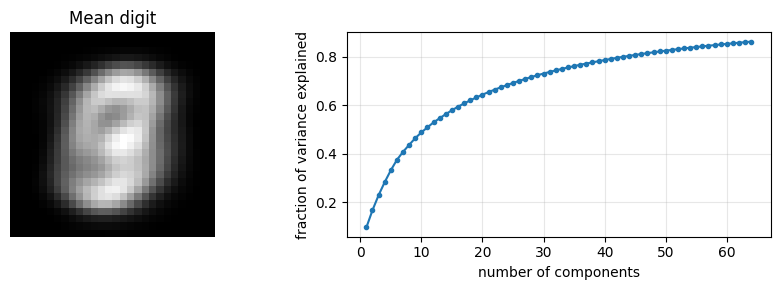
The mean digit is a fuzzy blur of all ten digits on top of each other. The variance curve rises steeply and then flattens: the first 10 components (out of 784 possible) already capture nearly half of all the variation among the digits, and 64 capture well over 80%.

Reconstruction with a few components¶

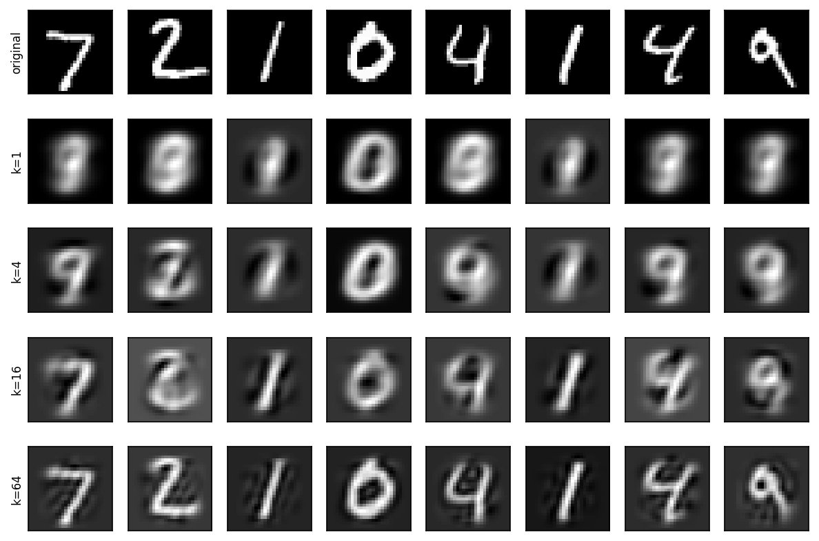
Let’s see what that means visually. We’ll take some test digits, which PCA never saw during fitting, project them onto the first $k$ components, and reconstruct: $\mathbf{x} \approx \boldsymbol{\mu} + \sum_{i<k} c_i \mathbf{v}_i$ .

which = np.arange(8)               # the first 8 test digits
coeffs = pca.transform(x_test[which])  # 8 x 64 coefficients

ks = [1, 4, 16, 64]
f, ax = plt.subplots(len(ks)+1, len(which), figsize=(8, 5.5))
for col, i in enumerate(which):
    ax[0, col].imshow(x_test[i].reshape(28, 28), cmap='gray')
    for row, k in enumerate(ks, start=1):
        rec = pca.mean_ + coeffs[col, :k] @ pca.components_[:k]
        ax[row, col].imshow(rec.reshape(28, 28), cmap='gray')
for row, label in enumerate(['original'] + [f'k={k}' for k in ks]):
    ax[row, 0].set_ylabel(label, fontsize=8)
for a in ax.ravel():
    a.set_xticks([]); a.set_yticks([])
plt.tight_layout()

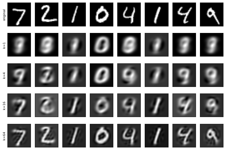
With a single component every digit is a variation on the blurry mean. By 16 components most digits are recognizable, and by 64 they’re quite clear, though still a little soft. That’s 64 numbers per digit instead of 784, more than a 12 $\times$ reduction. This is transform coding again, exactly as with JPEG, but with a basis tailored to the data.

The digits in PCA space¶

Finally, since the first two coefficients are the two most informative numbers about each digit, we can scatter every test digit in the plane by its first two coefficients, colored by its true label.

Xt = pca.transform(x_test)

plt.figure(figsize=(6,5))
sc = plt.scatter(Xt[:, 0], Xt[:, 1], c=y_test, cmap='tab10', s=2, alpha=.5)
plt.colorbar(sc, ticks=range(10), label='digit')
plt.xlabel('PC 1 coefficient')
plt.ylabel('PC 2 coefficient')
plt.title('MNIST test digits, first two principal components');

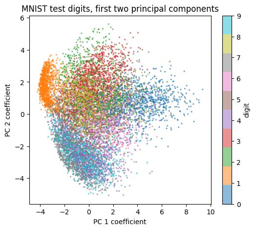
Some digits occupy their own regions. The 0s and 1s, for example, sit at opposite ends of the first component, and remember PCA was never told the labels. Others overlap heavily in these two dimensions. Two numbers per digit just aren’t enough to separate all ten classes. That’s a big part of why we’ll turn to classifiers that learn which directions matter for telling digits apart, rather than for describing them, which is all PCA optimizes.