Sampling and Spatial Resolution - imageprocessing-awesome

stough 202-

Preview: Sampling and Spatial Resolution

One of the core properties of any digital image is its resolution. But this is a very loaded word in that it is used in a variety of ways for different purposes. Very generally, the light from the external world comes at our digital camera from a virtually uncountably infinite number of directions, with each direction specifying a “color” among a virtually uncountably infinite number of color distributions and intensities. Resolution broadly refers to the finite sampling of this infinite world. In the case of spatial resolution that is simply the number of pixels or “picture elements” that our camera can possibly obtain (see “internal image plane” below). Beyond spatial resolution, there is also color resolution, which we get to elsewhere.

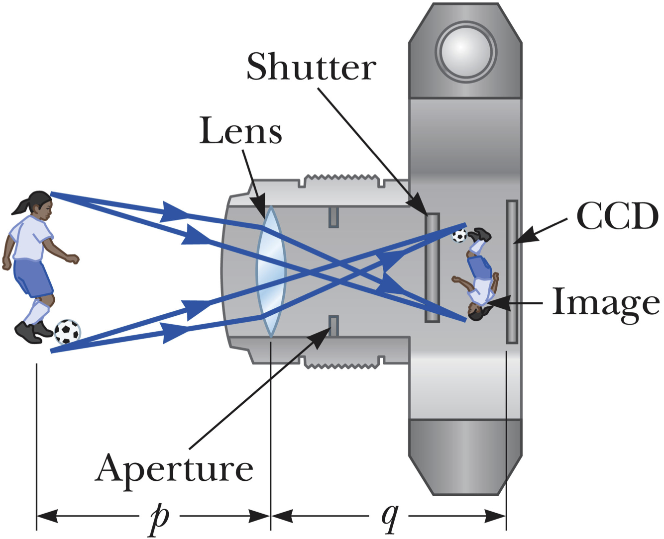
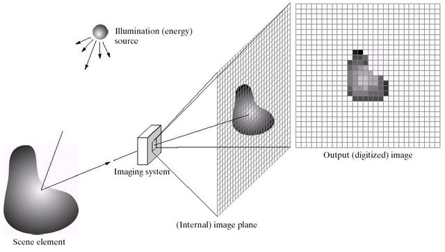
In this notebook we’re going to look at the spatial resolution of a digital image.

Imports¶

We’ll use the rescale method in the powerful scikit-image module in order to change image resolution. We’ll also be using some widgets to put together an interactive visualization. Lastly, we’re starting to import common functionality from our own ../dip_utils/ utilities folder.

%matplotlib inline
import matplotlib.pyplot as plt
import numpy as np
from skimage.transform import rescale
from ipywidgets import VBox, IntSlider, AppLayout

# For importing from alternative directory sources
import sys  
sys.path.insert(0, '../dip_utils')

# Importing from our own utilities
from matrix_utils import arr_info
from vis_utils import vis_image, vis_pair

I = plt.imread('../dip_pics/grandCanyon.jpg')
arr_info(I)

((2160, 3840, 3), dtype('uint8'), np.uint8(0), np.uint8(255))

vis_image(I, figsize=(5,3))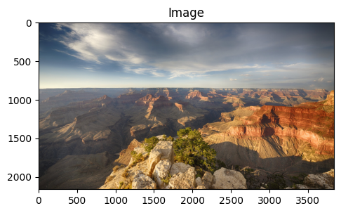

As you can see the image matrix I is 2160 rows by 3840 columns, with three color channels (red, green, blue) in the integer range $[0,255]$ . By the way this is literally a “4K” image.

“4K” refers to the approximate number of columns, or the left-right sampling of the image. At an aspect ratio of 16(width, columns):9(height, rows), a “1080” high definition image or screen is 1920 pixels across, about 2K. So a 4K is a 2x2 grid of such 2K screens. It has 4 times the number of pixels in a 2K (or 1080). It’s more complicated than that, but not by much.

If we think of an image as a grid of pixels, where the center of each pixel represents that pixel’s coordinates, then changing the resolution of an image involves resampling the space between those pixel coordinates. We’ll avoid most of the math here by relying on skimage, but take a very simple example: If we wanted to halve the number of pixels both in width and height without cropping, we could just take the average of every non-overlapping 2x2 pixel patch. Similarly, if we wanted to double the number of pixels in both directions, we could simply make a 2x2 grid of copies of each pixel.

We’ll start by doing this halving of resolution. We’ll first ask rescale to give us an image with 1/4 the number of pixels. But then we’ll upsample that image by four. The order and anti-aliasing parameters are used to define the level of “smoothing” that takes place, i.e. how many neighboring pixels to consider when deciding the color of the new sample coordinate.

# The image is so large, take a tiny piece of it to test the order, anti-aliasing parameters.
# I = I[800:930, 1900:2050, :]

sI = rescale(I, .25,
             order=0, # use nearest neighbor sampling
             anti_aliasing=False,
             channel_axis=-1)

# rescale back up
reI = rescale(sI, 4,
              order=0, # use nearest neighbor sampling
              anti_aliasing=False,
              channel_axis=-1)

vis_pair(I, reI, first_title='Original', second_title='Quarter Res')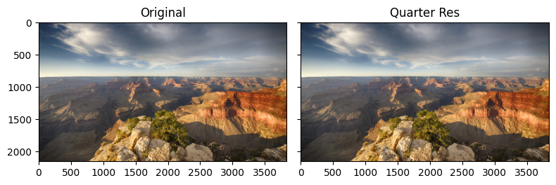

If you’re displaying this notebook in anything less than 8K full screen it’s likely that the original and quarter-resolution images look identical. Use the zoom function to look more closely at particular areas to observe the difference. As you zoom in you should start to see the pixels that make up both images, and you will see the difference in spatial resolution. In this display, the reason I upsample the just downsampled image is so that the two image axes are ‘shared’ and interacting with one causes the same interaction in the other (like zooming).

Below is an interactive visualization that allows you to select the degree of downsampling in the right-hand image. First, we’ll define a quick function that does the resampling.

def downandup(I, factor):
    # downscale
    sI = rescale(I, 1/factor,
                 order=0, # use nearest neighbor
                 anti_aliasing=False,
                 channel_axis=-1)

    # rescale back up
    reI = rescale(sI, factor,
                  order=0, # use nearest neighbor sampling
                  anti_aliasing=False,
                  channel_axis=-1)
    return reI

pass  # (static) plt.ioff()

# Create a slider object
slider = IntSlider(
    orientation='horizontal',
    description='Exponent:',
    value=0,
    min=0,
    max=10
)

slider.layout.margin = '0px 30% 0px 30%'
slider.layout.width = '40%'


f, ax = plt.subplots(1,2, figsize=(10,3), sharex=True, sharey=True)
f.canvas.header_visible = False
ax[0].imshow(I, interpolation='none')
ax[0].set_title('Original')

rdisp = ax[1].imshow(I, interpolation='none')
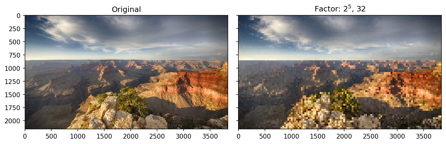
rtext = ax[1].set_title(rf'Factor: $2^{slider.value:d}$, {2**slider.value:d}')


# A function that will be called whenever the slider changes.
def update(change):
    Ire = downandup(I, factor=2**slider.value)
    rdisp.set_data(Ire)
    rtext.set_text(rf'Factor: $2^{slider.value:d}$, {2**slider.value:d}')
    f.canvas.draw()
    f.canvas.flush_events()

# Connecting the slider object to the update function above.
# This is event-handling.
slider.observe(update, names='value')

plt.tight_layout()
# Creates an application interface with the various 
# pieces we already instantiated inside of it. 
pass  # (static) AppLayout(
pass  # (static)     center=f.canvas,
pass  # (static)     footer=slider,
pass  # (static)     pane_heights=[0, 6, 1]
pass  # (static) )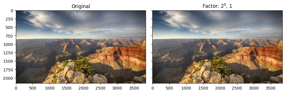

Note that I’m using the slider.value as an exponent to give a little more effect. Think of the printed “Factor” ( $2^{slider.value}$ ) as the number of pixels to combine in each dimension. So at an exponent of 3, we’re scaling the image by 8 in each dimension; i.e., each pixel in the downsampled image represents 64 pixels in the original.

Note you could also modify the parameters we send to rescale, such as turning on anti-aliasing, and seeing what that does to the output.

🧠 Further Efforts¶

Now that you’ve seen how spatial resolution affects image quality, compare some of the ways the resampling itself can be done.

Compare interpolation methods. The order argument to rescale decides how a new pixel’s value is computed from the old ones: 0 is nearest neighbor (what we used), 1 is bilinear, and 3 is bicubic. Try each one for both the downsampling and the upsampling in downandup(). Which order gives a blocky result, and which gives a blurry one? Which looks most like the original at a factor of 8?
Guidance: Give downandup() an order parameter instead of editing the constants, so you can compare two orders side by side with vis_pair. Zoom in on edges and fine texture. Higher orders are also slower on this 4K image, so test on the small crop suggested in the commented-out line near the top.
Turn on anti-aliasing. Set anti_aliasing=True in the downsampling call and compare against False at a large factor. What artifacts go away, and what does it cost you?
Guidance: Anti-aliasing smooths the image before sampling it. Look for patterns that weren’t in the original, such as jagged diagonal edges or moiré in finely repeated texture. We’ll see why smoothing first helps in low-pass filtering and, more precisely, in the Fourier chapter.