Color Quantization - imageprocessing-awesome

stough 202-

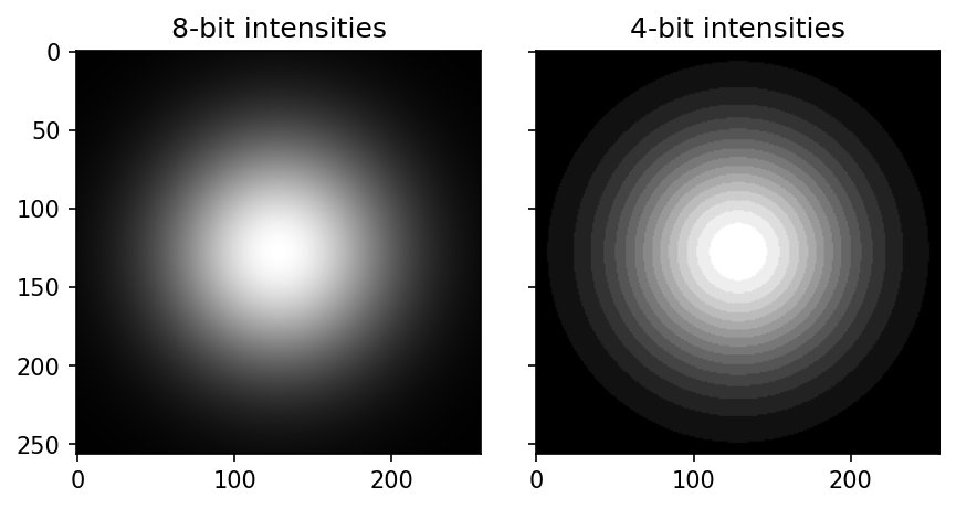
Quantization is how we map an otherwise continuous range of values into the finite discrete set that we can store. We have seen that most commmonly we use 8-bit values in the range $[0,255]$ to represent all possible intensities, a continuous range in reality.

We’ll observe this quantization on a single-channel grayscale image to start.

Imports¶

We’re adding scipy.stats.norm as a function for plotting a Gaussian.

%matplotlib inline
import matplotlib.pyplot as plt
import numpy as np
from scipy.stats import norm

# For importing from alternative directory sources
import sys  
sys.path.insert(0, '../dip_utils')

import matrix_utils
from vis_utils import vis_image, vis_pair

A nice way to make a Gaussian image: make a 1D sampled Gaussian and take its outer product. Then we’ll normalize it to a $[0,255]$ 8-bit integers.

x = np.linspace(-2.5,2.5,257)

plt.figure(figsize=(4,2))
plt.plot(x, norm.pdf(x))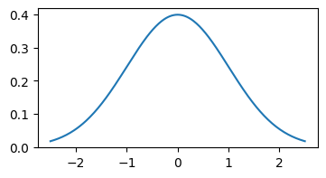

I = np.outer(norm.pdf(x),norm.pdf(x))
I = I/I.max()
I = np.uint8(255*I +.5)

matrix_utils.arr_info(I)

((257, 257), dtype('uint8'), np.uint8(0), np.uint8(255))

# Note that we can a utility rather than always type these out.
# plt.figure(figsize=(4,4))
# plt.imshow(I, cmap='gray', interpolation=None);
vis_image(I, cmap='gray')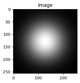

The above is a Gaussian blob image, as continuous as we can normally make it, in what’s called 8-bit depth. Zoom in and see just how smooth it is. We can also plot the original continuous Gaussian. We’ll plot with two y axes using matplotlib.

f, ax1 = plt.subplots(figsize=(7,3))
ax1.scatter(x, norm.pdf(x), c='blue')

ax2 = ax1.twinx()
plt.bar(x, I[128,:], fill=False, width = np.diff(x)[0], edgecolor='red');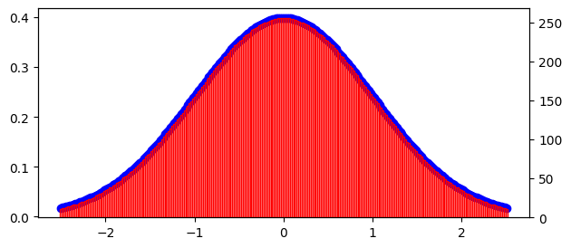

The complicated plot above shows in blue dots the continuous value of the Gaussian at the location, while the red bars show the 8-bit value of the sampled image (that is, sampling from a horizontal line, I[128,:], right through the middle of the image). In the current image there are 256 possible intensities. We can quantize the intensities to a bit depth of less than 8 by ignoring the low-order bits in the intensity. This is analogous to dividing by 10 and ignoring the fractional part; since the numbers are stored in binary, bit-shift to the right by 1 is equivalent to dividing by 2. Let’s try 4 bit intensity (that is, divide by 2 four times, or in total divide by 16).

I4 = (I >> 4)

# Again, why not use a utility:
# f, ax = plt.subplots(1,2, figsize=(6,3), sharex=True, sharey=True)

# ax[0].imshow(I, cmap='gray', interpolation=None)
# ax[0].set_title('8-bit intensities')

# ax[1].imshow(I4, cmap='gray', interpolation=None)
# ax[1].set_title('4-bit intensities')

# [a.axes.get_xaxis().set_visible(False) for a in ax];
# [a.axes.get_yaxis().set_visible(False) for a in ax];
# plt.tight_layout()
vis_pair(I, I4, first_title='8-bit intensities', 
         second_title='4-bit intensities', cmap='gray',
         figsize=(6,3))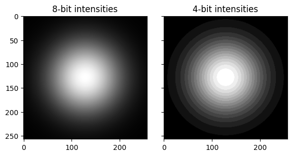

We can try the same 1D plot as we did before, to see how far off our I4 intensities are from the continuous original.

f, ax1 = plt.subplots(figsize=(7,3))
ax1.scatter(x, norm.pdf(x), c='blue')

ax2 = ax1.twinx()
plt.bar(x, I4[128,:], fill=False, width = np.diff(x)[0], edgecolor='red');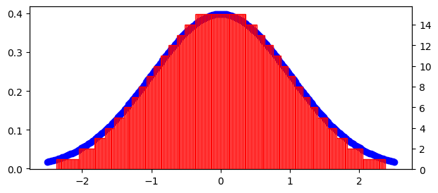

We’ve gotten all this way in a demo on “color quantization” and we haven’t seen any color yet. Oh well, I leave it to you.

🔨 Your Turn: Interactive Color Quantization¶

Bit depth is easiest to appreciate when you can drag it down and watch an image fall apart, so let’s build that.

Task: Make an interactive figure that shows a color image next to a copy quantized to a bit depth chosen with a slider, from 8 bits down to 1 bit per channel. Use ../dip_pics/sf.jpg or an image of your own. At what bit depth do you first notice the change, and where in the image do you notice it first?

Guidance:

Model the figure on the slider demos in spatial resolution and interactive visualization: plt.ioff(), a figure, an IntSlider, an update function that calls set_data on the displayed image, slider.observe(update, names='value'), and finally VBox([slider, fig.canvas]).
Quantize each channel the way we did the gray image above, by shifting off low-order bits. Check with arr_info that the image really is uint8 first.
After shifting right by $k$ bits, the values are in a smaller range like $[0, 15]$ , which imshow would display as nearly black. imshow needs a 3-channel image as floats in $[0,1]$ or integers in $[0,255]$ , so scale the result back up before displaying it.

🧠 Further Efforts¶

Once you have the interactive figure working, look more carefully at what quantization loses.

Map the quantization error. Display the difference between the original image and a quantized version (scaled back to the same range) as an image, for a few bit depths. Where in the image is the error largest, and how does the largest possible error depend on the bit depth?
Guidance: Convert to a signed or float type before subtracting, or uint8 arithmetic will wrap around. A grayscale display of the error magnitude with a colorbar is easiest to read.
Watch the histogram. Plot the histograms of the original and quantized images with vis_hists (from vis_utils). How many distinct values remain at each bit depth?
Guidance: np.unique counts distinct values directly; check that it agrees with the histogram.
One channel at a time. Quantize only the red channel, then only the green, then only the blue, leaving the others at 8 bits. Is the loss equally visible in each?
Guidance: Recall from the Color chapter that our eyes are not equally sensitive to all three. Try a photograph with large smooth regions, like a sky.
Different kinds of images. Compare a natural photograph, a cartoon or logo, and the Gaussian blob from this notebook. Which survives low bit depths best?
Guidance: Think about where the false contours appear: in smooth gradients or at sharp edges?

Going further¶

Dithering. Instead of rounding every pixel the same way, dithering chooses different quantizations for neighboring pixels, or spreads each pixel’s rounding error onto its neighbors (Floyd–Steinberg). Try implementing Floyd–Steinberg on the gray Gaussian blob at 1 or 2 bits and compare it with plain quantization, from up close and from across the room.
Non-uniform quantization. We spaced our quantization levels evenly. Try spacing them unevenly, for example closer together in the dark range, and compare at the same number of levels. (The power transforms of the Enhancement chapter show why that might help.)