Heightmap Demo - imageprocessing-awesome

stough 202-

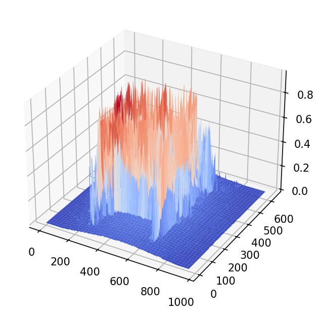
In this quick demo I wanted to show how an image can be seen as a height-map, where the xy-plane is the domain of the image, while the z-axis represents the image intensity. This is easy enough with matplotlib’s 3D plotting capability. Specifically I would refer you to the surface plot examples.

Why bother? Because thinking of an image as terrain is one of the most useful mental models in this book. Bright regions are plateaus, dark regions are valleys, and edges are cliffs. Later, when we filter images, blurring will mean eroding the terrain smooth, and finding edges will mean measuring how steep the slope is.

%matplotlib inline
import matplotlib.pyplot as plt
from matplotlib import cm
from mpl_toolkits.mplot3d import Axes3D
import numpy as np
from skimage import color

# For importing from alternative directory sources
import sys  
sys.path.insert(0, '../dip_utils')

from matrix_utils import arr_info
from vis_utils import vis_image

I = color.rgb2gray(plt.imread('../dip_pics/D_image.jpg'))

arr_info(I)

((960, 640), dtype('float64'), np.float64(0.0), np.float64(0.9521090196078432))

vis_image(I, cmap='gray')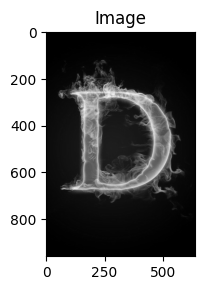

X, Y = np.meshgrid(range(0,I.shape[0]), range(0,I.shape[1]), indexing='ij')

fig = plt.figure(figsize=(5,5))
ax = fig.add_subplot(111, projection='3d')

ax.plot_surface(X, Y, I, cmap=cm.coolwarm);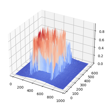

The argument projection='3d' means the ax returned is an Axes3D object. We then call that object’s plot_surface method with a colormap so that the colors change as a function of the image intensity, or z coordinate.

Note also that 3D plotting normalizes the units for a square output, even while the original image may not be. Lastly, code that does this surface plotting has been added to vis_utils as vis_surface if we need it in the future.

One more subtle thing: our image is $960 \times 640$ , but the surface above looks fairly coarse. That’s because plot_surface quietly samples the data down to at most 50 rows and 50 columns by default (its rcount and ccount arguments), so that the 3D rendering stays fast. That’s a reduction in spatial resolution, exactly the subject of this chapter. You can ask for more with, e.g., rcount=200, ccount=200, at the cost of a slower, laggier interactive plot.

Smoothing the Terrain¶

As a preview of where we’re headed, let’s blur the image a bit (each pixel replaced by a weighted average of its neighbors, which we’ll study in spatial filtering) and look at the terrain again. I’ll also downsample by 8 in each dimension first, so we can see more of the surface’s detail with fewer points.

from scipy.ndimage import gaussian_filter

Is = I[::8, ::8]                    # 120 x 80
Ib = gaussian_filter(Is, sigma=2)   # blurred

Xs, Ys = np.meshgrid(range(Is.shape[0]), range(Is.shape[1]), indexing='ij')

fig = plt.figure(figsize=(8,4))
for k, (Z, title) in enumerate([(Is, 'downsampled'), (Ib, 'downsampled + blurred')]):
    ax = fig.add_subplot(1, 2, k+1, projection='3d')
    ax.plot_surface(Xs, Ys, Z, cmap=cm.coolwarm, rcount=120, ccount=80)
    ax.set_zlim(0, 1)
    ax.set_title(title)
plt.tight_layout()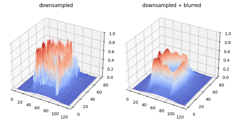

The jagged peaks of the smoke have been worn down into rolling hills, and the cliffs at the edge of the letter now slope more gently. Keep this picture in mind: smoothing lowers slopes, and edges are where the slopes are steep.