Using Fourier Transform for Blurring, Sharpening

stough 202-

DIP 4.7 shows similar.

We saw in fft_intro that we can denoise an image in the Fourier space, also called the frequency domain. We also saw that we can consider the magnitude and phase components separately given the Fourier Transform of an image. Here we’re going to play around further in the Fourier domain and show how we can blur and sharpen an image through clever manipulation in the frequency domain.

Imports¶

We’ll use the Fast Fourier Functions again.

%matplotlib inline
import matplotlib.pyplot as plt
from matplotlib.colors import LogNorm
from skimage.color import rgb2gray
import numpy as np

# For importing from alternative directory sources
import sys  
sys.path.insert(0, '../dip_utils')

from matrix_utils import (arr_info,
                          make_linmap)
from vis_utils import (vis_rgb_cube,
                       vis_hists,
                       vis_image,
                       vis_pair,
                       vis_surface)

from scipy.fft import (fft2, ifft2, fftshift, 
                       ifftshift, fftn, ifftn)
from skimage.transform import resize

Blur, Edginess, Sharpen¶

In this worksheet we’ll take an image and manipulate it in the frequency space.

Use fftn to convert to the Fourier domain
Scale and manipulate the spectrum coefficients in the Fourier domain.
Use ifftn to convert back to the image/spatial domain.

Of note in this exercise is that visualization can be a bear. We’ll use fftshift to visualize the Fourier domain in a way that shows the low-frequency components in the center of the image and higher frequencies out towards the extremes.

I = plt.imread('../dip_pics/switzerland_hazy.jpg')
I = I/255.0
arr_info(I)

((1536, 2048, 3), dtype('float64'), np.float64(0.0), np.float64(1.0))

vis_image(I, show_ticks=False)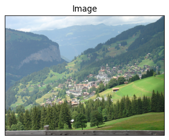

I_fft = fftn(I)

arr_info(I_fft)

((1536, 2048, 3),
 dtype('complex128'),
 np.complex128(-231815.0537404591-282716.775763718j),
 np.complex128(4825197.364705882-0j))

One subtlety: fftn transforms along every axis, so on our $1536 \times 2048 \times 3$ color image it also takes a (tiny, 3-point) Fourier transform across the color channels. Everything we do below scales the spectrum the same way for all three of those color “frequencies”, so the result is exactly the same as filtering each channel separately with a 2D FFT. If you want to be explicit, fft2(I, axes=(0,1)) transforms only the two spatial axes.

Visualizing in the Fourier domain¶

A bit difficult artifact about fft is that the output places the lower-frequency coefficients at the corners of the transform array. Normally however, we wish to visualize the spectrum such that lower frequencies are in the center of the figure. We’ll use fftshift to do this.

# Visualize the freq domain.
temp = np.abs(I_fft)
temp = np.log2(1 + temp)/np.log2(1+temp.max())
vis_image(fftshift(temp))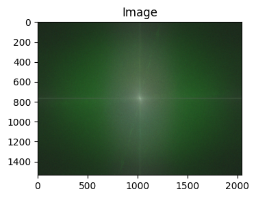

Using a Gaussian for smooth scaling¶

In fft_intro we simply zero’d out all the coefficients outside of some square in the fourier space in order to eliminate high-frequency content. However this can lead to weird artifacts called ringing (the Gibbs phenomenon): ripples alongside strong edges, caused by the abrupt cutoff. The proper way to manipulate the fourier domain is through smoother scaling, like the Gaussian. Below we’ll define a function that generates a 2D Gaussian of the same shape as an input image. We did something like this using scipy’s norm and np.outer in color_quantization. Here, we give ourselves a little more flexibility by directly evaluating the Gaussian exponential at all the pixel coordinates we want.

\mathcal{N}(\mu, \sigma)(x) = e^{-(x-\mu)^2/2\sigma^2}

(1)

# Thanks https://stackoverflow.com/questions/29731726/how-to-calculate-a-gaussian-kernel-matrix-efficiently-in-numpy

def gaussian(I, sig):
    x, y = np.meshgrid(np.arange(I.shape[1]), np.arange(I.shape[0]))
    coords = np.stack([x,y], axis=-1)
    c = np.reshape([I.shape[1]/2, I.shape[0]/2], (1,1,2))
    return np.exp((-(np.linalg.norm(coords-c, axis=2)**2))/(2*sig**2))

vis_image(gaussian(I, 200))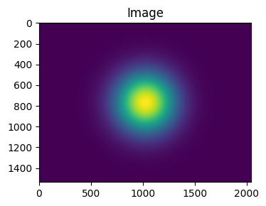

Blur: Use the Gaussian as a scalar multiple in the frequency domain¶

Great reference for matplotlib surface visualizations. Here I just want to visualize what the scalar we’ll use looks like over the image, as a surface in 3D.

vis_surface(gaussian(I, 200))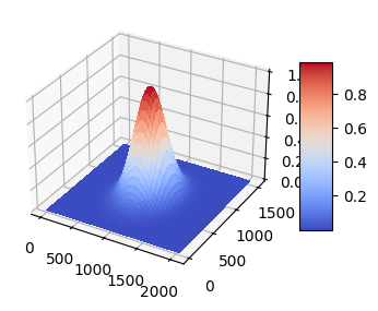

The Actual scaling in frequency space¶

We want to multiply the Fourier coefficients of the image by this Gaussian image, thereby scaling the coefficients. We just have to remember that I_fft needs to be fftshift’d to make the pixels line up correctly. We only do the shifting for visualization until now. Note that the variable temp comes from several cells ago, when we first visualized I_fft.

vis_pair(fftshift(temp), gaussian(I, 100), 
         first_title='Fourier Spectrum of Image', 
         second_title='Gaussian Scaling Factor',
         show_ticks=False)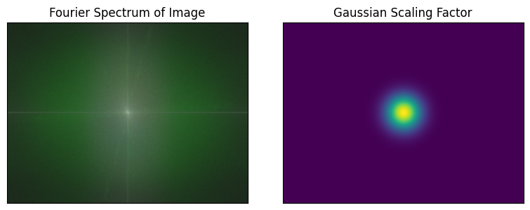

blur_I_fft = ifftshift(np.multiply(fftshift(I_fft), gaussian(I, 100)[...,None]))

# Visualize the freq domain.
temp = np.abs(blur_I_fft)
temp = np.log2(1 + temp)/np.log2(1+temp.max())
vis_image(fftshift(temp))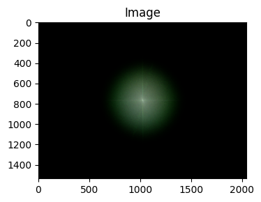

Now, we’ll invert the fourier transform to go back to image space.

I_blurred = ifftn(blur_I_fft)
arr_info(I_blurred)

((1536, 2048, 3),
 dtype('complex128'),
 np.complex128(0.07292675544127314-2.752391556703007e-18j),
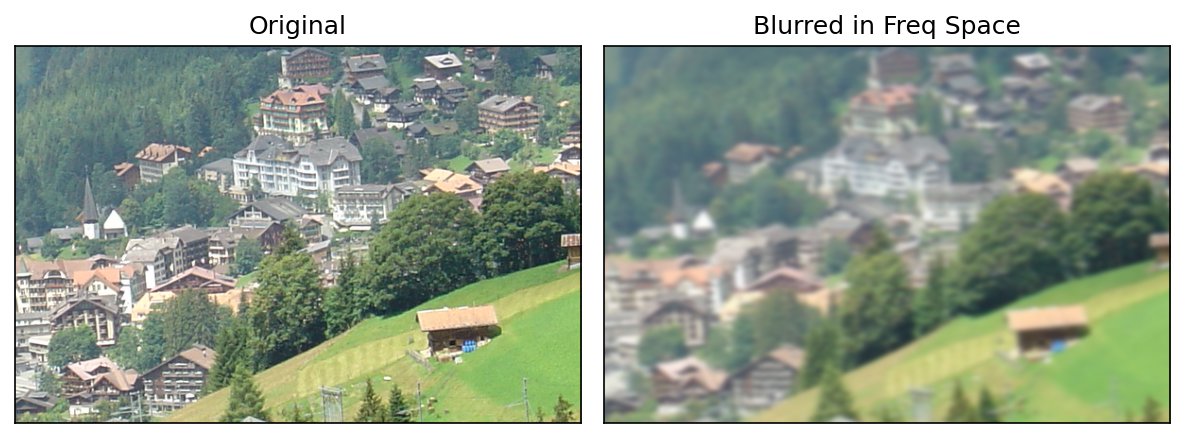
 np.complex128(0.9999999999765902+1.777827989816071e-18j))

vis_pair(I, np.clip(I_blurred.real, 0, 1), second_title='Blurred in Freq Space', show_ticks=False)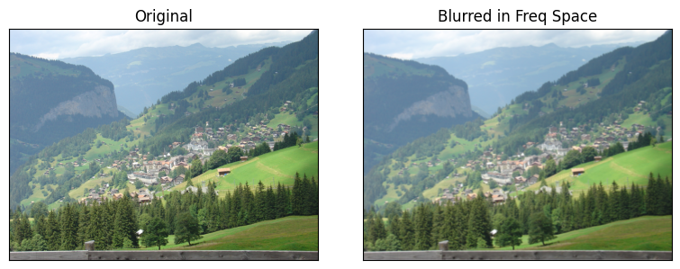

The blur is gentle: the fine texture of the trees and village is softened, but the overall scene is intact. The center of the spectrum, the low frequencies, is multiplied by nearly 1 and passes through untouched, while frequencies farther out are increasingly suppressed.

The Convolution Theorem¶

Here’s the deep connection between this notebook and spatial filtering. The convolution theorem says that convolving an image with a kernel in the spatial domain is exactly the same as multiplying their Fourier transforms:

\mathcal{F}\{f * h\} = \mathcal{F}\{f\} \cdot \mathcal{F}\{h\}

So multiplying the spectrum by our Gaussian was a convolution with some spatial kernel: the one whose Fourier transform is that Gaussian. And the Fourier transform of a Gaussian is another Gaussian, with its width inverted. A Gaussian of standard deviation $\sigma_f$ in frequency corresponds to a spatial Gaussian of standard deviation

\sigma_s = \frac{N}{2\pi\sigma_f}

along an axis of $N$ pixels. A narrow window in frequency (keep only the very lowest frequencies) means a wide blur in space, and vice versa. Our image isn’t square, so the same $\sigma_f = 100$ gives a slightly different $\sigma_s$ along each axis. Let’s check by blurring the image directly with scipy.ndimage.gaussian_filter. One detail: the FFT treats the image as if it repeats periodically, so to match exactly we tell gaussian_filter to wrap around at the borders.

from scipy.ndimage import gaussian_filter

sig_f = 100
H, W = I.shape[:2]
sig_s = (H/(2*np.pi*sig_f), W/(2*np.pi*sig_f), 0)   # no blurring across color channels
print(f'Equivalent spatial sigmas: {sig_s[0]:.2f} rows, {sig_s[1]:.2f} columns')

I_spatial = gaussian_filter(I, sigma=sig_s, mode='wrap', truncate=6)
print('Largest difference from the frequency-domain blur:', np.abs(I_spatial - I_blurred.real).max())

Equivalent spatial sigmas: 2.44 rows, 3.26 columns

Largest difference from the frequency-domain blur: 2.9446101112995393e-10

Identical, up to floating-point round-off. Two routes to the same blur: a weighted average of a small neighborhood in space, or a multiplication in frequency. Which is faster depends on the kernel size. A small kernel is cheap to apply directly, but the cost of direct convolution grows with the kernel’s area, while the FFT route costs about the same no matter how wide the blur.

This also explains the earlier comparison between box and Gaussian blurs. The Fourier transform of a box is a $\text{sinc}$ function, which ripples, with lobes that go negative and back again at higher and higher frequencies. So a box blur doesn’t steadily suppress high frequencies: it lets some of them back through, flipped in sign. The Gaussian’s transform just falls off smoothly.

Edge Finder: Use the complement of the Gaussian as the scalar¶

Thereby keeping only the higher frequency content.

vis_surface(1-gaussian(I, 200))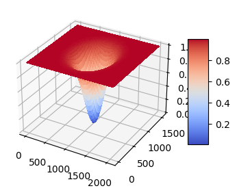

edge_I_fft = ifftshift(np.multiply(fftshift(I_fft), 1-gaussian(I, 100)[...,None]))

# Visualize the freq domain.
temp = np.abs(edge_I_fft)
temp = np.log2(1 + temp)/np.log2(1+temp.max())
vis_image(fftshift(temp))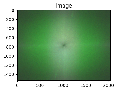

I_edges = ifftn(edge_I_fft)
arr_info(I_edges.real)

((1536, 2048, 3),
 dtype('float64'),
 np.float64(-0.5787901883732011),
 np.float64(0.6158012435677704))

temp = np.abs(I_edges.real)
temp = (temp - temp.min())/(temp.max()-temp.min())
arr_info(temp)

((1536, 2048, 3), dtype('float64'), np.float64(0.0), np.float64(1.0))

vis_pair(I, temp, second_title='Just High Freq', show_ticks=False)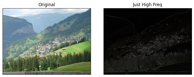

Using $1 - \text{Gaussian}$ keeps the high frequencies and suppresses the low ones, a high-pass filter. The result is dark wherever the image is smooth, including the sky, the haze, and the broad slopes, and bright only at fine detail and edges: the rooftops, the tree line, the ridge. It’s the frequency-domain cousin of the Laplacian. Notice that the low-pass and high-pass scalings add up to exactly 1, so I_blurred + I_edges gives back the original image: we’ve split the image into its smooth part and its detail.

🔨 Your Turn: Sharpen in the Frequency Domain¶

We’ve blurred the image by scaling its spectrum with a Gaussian, and isolated its detail by scaling with one minus a Gaussian. How might we potentially sharpen the image?

Task: Sharpen I by scaling its Fourier transform, and show the original and sharpened images side by side. Plot your scaling factor as a surface, the way we did for the Gaussian, and explain its shape.

Guidance:

Recall unsharp masking in the spatial domain: the original image plus some multiple of its detail. You already have both of those here.
The Fourier transform is linear: the transform of a sum of images is the sum of their transforms, and the transform of $k$ times an image is $k$ times its transform. So you can do all of your work as one multiplication in the frequency domain. What single scaling factor would do it?
As above, the factor is built centered, so fftshift the transform before multiplying and ifftshift it after. Take .real of the inverse transform, and np.clip to $[0,1]$ for display.
Try a few amounts of sharpening and a few Gaussian widths. Zoom in on the village and the trees to compare.