The Discrete Fourier Transform - imageprocessing-awesome

DRAFT, not finalized. This chapter is new and still under review.

stough 202-

Complex exponentials: rotating arrows
The DFT as a change of basis
Magnitude and phase
Sampling and aliasing
The fast Fourier transform
On to two dimensions
🔨 Your Turn: Find the Hidden Tones
🧠 Further Efforts

In the BlockTransform chapter we described image blocks as combinations of patterns, and the DCT in particular describes a signal as a sum of sampled cosines of increasing frequency. The discrete Fourier transform (DFT) is the DCT’s older, more famous relative. It also describes a signal as a sum of waves of increasing frequency, but its waves are complex exponentials, which carry both a cosine and a sine. That makes it handle one thing especially gracefully: shifts. Where a wave starts, its phase, gets a number of its own.

In this notebook we’ll build up the 1D DFT from scratch: what its basis vectors look like, what its coefficients mean, what goes wrong when we sample too coarsely, and how the fast Fourier transform (FFT) computes it so quickly. Then Fast Fourier Analysis takes it to images.

%matplotlib inline
import matplotlib.pyplot as plt
import numpy as np
import time

# For importing from alternative directory sources
import sys
sys.path.insert(0, '../dip_utils')

from matrix_utils import arr_info
from wavelet_utils import make_dct_matrix

Complex Exponentials: Rotating Arrows¶

A complex number $z = a + bj$ is a point in the plane, $a$ along the real axis and $b$ along the imaginary. (Engineers, and Python, write $j$ for $\sqrt{-1}$ , since $i$ is taken by current; Python spells it 1j.) The key fact is Euler’s formula:

e^{j\theta} = \cos\theta + j\sin\theta,

the point at angle $\theta$ on the unit circle. As $\theta$ grows, $e^{j\theta}$ runs around the circle, like the tip of a rotating arrow, or phasor. Its real part traces out a cosine and its imaginary part a sine.

The DFT’s basis vectors sample such a rotation at $N$ evenly spaced steps. For frequency $k$ , the $n$ -th sample is

w_k[n] = e^{2\pi j\,kn/N}, \qquad n = 0, 1, \ldots, N-1,

which steps $k/N$ of the way around the circle each time, and so goes around exactly $k$ times in $N$ samples.

N = 16
n = np.arange(N)

fig, ax = plt.subplots(2, 2, figsize=(9, 6), gridspec_kw={'width_ratios': [1, 1.8]})
for row, k in enumerate([1, 3]):
    w = np.exp(2j * np.pi * k * n / N)
    # Left: the samples as points on the unit circle, numbered by n.
    ax[row, 0].plot(np.cos(np.linspace(0, 2 * np.pi, 200)), np.sin(np.linspace(0, 2 * np.pi, 200)), 'k:', lw=0.8)
    ax[row, 0].plot(w.real, w.imag, 'o')
    for i in range(6):
        ax[row, 0].annotate(str(i), (w[i].real, w[i].imag), xytext=(6, 4), textcoords='offset points')
    ax[row, 0].set_aspect('equal')
    ax[row, 0].set_title(f'$w_{k}[n]$ in the complex plane (n = 0..5 labeled)', fontsize=9)
    ax[row, 0].set_xlabel('real'); ax[row, 0].set_ylabel('imaginary')
    # Right: the real and imaginary parts as signals.
    ax[row, 1].stem(n, w.real, linefmt='C0-', markerfmt='C0o', basefmt=' ', label='real part (cosine)')
    ax[row, 1].stem(n + 0.15, w.imag, linefmt='C1-', markerfmt='C1o', basefmt=' ', label='imaginary part (sine)')
    ax[row, 1].set_title(f'k = {k}: {k} full turn{"s" if k > 1 else ""} in N = {N} samples', fontsize=9)
    ax[row, 1].legend(fontsize=7, loc='upper right')
plt.tight_layout()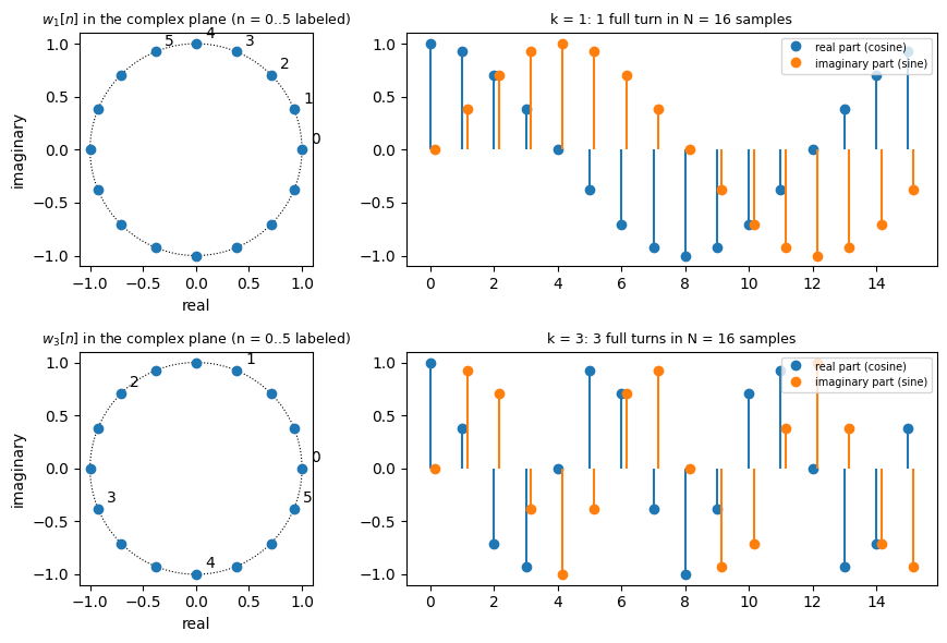

For $k = 1$ (top), the samples step one sixteenth of the way around the circle each time, counterclockwise, so the real part is one period of a cosine and the imaginary part one period of a sine. For $k = 3$ (bottom), each step is three sixteenths of a turn, so the samples go around three times and the cosine and sine have three periods. Higher $k$ means faster rotation: higher frequency.

The DFT as a Change of Basis¶

The DFT of a signal $x$ of length $N$ measures how much of each frequency $k = 0, \ldots, N-1$ the signal contains, by taking its inner product with each $w_k$ :

X[k] = \sum_{n=0}^{N-1} x[n]\, e^{-2\pi j\,kn/N}.

(For complex vectors, the inner product conjugates one of them, which is where the minus sign in the exponent comes from.) Just like make_dct_matrix, we can collect these as the rows of an $N \times N$ matrix $\mathbf{F}$ , with $F_{kn} = e^{-2\pi j\,kn/N}$ , so that the whole transform is one matrix-vector product, $X = \mathbf{F}x$ .

def dft_matrix(N):
    k = np.arange(N).reshape(-1, 1)    # rows: frequency
    n = np.arange(N).reshape(1, -1)    # columns: sample
    return np.exp(-2j * np.pi * k * n / N)

F = dft_matrix(8)
D = make_dct_matrix(8)

fig, ax = plt.subplots(1, 3, figsize=(10, 3.2))
for a, M, title in zip(ax, [D, F.real, F.imag], ['DCT matrix', 'DFT matrix, real part', 'DFT matrix, imaginary part']):
    a.imshow(M, cmap='gray')
    a.set_title(title, fontsize=10)
    a.set_xlabel('n'); a.set_ylabel('k')
plt.tight_layout()

x = np.random.random(8)
print('F @ x matches np.fft.fft(x):', np.allclose(F @ x, np.fft.fft(x)))
print('F F^H = N I:', np.allclose(F @ F.conj().T, 8 * np.eye(8)))

F @ x matches np.fft.fft(x): True
F F^H = N I: True

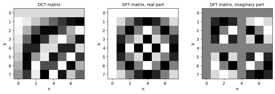
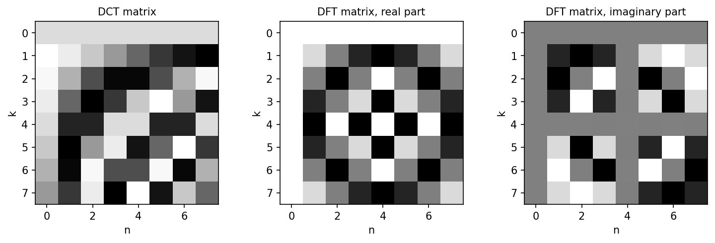
Each row of the DFT matrix is one sampled wave: the real part (middle) holds the cosines and the imaginary part (right) the negated sines. Row $k = 0$ is constant, so $X[0]$ is just the sum of the signal. Compared with the DCT (left), the rows’ frequencies rise until the middle row, $k = N/2$ , and then fall again. More on that symmetry below.

The first printed check confirms that our matrix computes exactly what NumPy’s np.fft.fft does. The second shows that the rows are orthogonal: $\mathbf{F}\mathbf{F}^H = N\mathbf{I}$ , where $\mathbf{F}^H$ is the conjugate transpose. So, like the DCT and Haar matrices, $\mathbf{F}/\sqrt{N}$ is an orthonormal (for complex matrices, unitary) basis, and the inverse transform is just the conjugate transpose:

x = \frac{1}{N}\mathbf{F}^H X, \qquad x[n] = \frac{1}{N}\sum_{k=0}^{N-1} X[k]\, e^{2\pi j\,kn/N}.

The DFT is a change of basis, from “the value at each sample” to “the amount of each frequency”, with nothing lost. (NumPy puts the whole $1/N$ in the inverse rather than $1/\sqrt{N}$ in each direction; that’s just bookkeeping.)

Magnitude and Phase¶

Each coefficient $X[k]$ is a complex number, and its polar form tells us two things: its magnitude $|X[k]|$ is how much of frequency $k$ is in the signal, and its phase $\angle X[k]$ is where that wave is shifted to. Let’s transform a signal with a known recipe: a constant 1, plus a cosine of amplitude 3 at frequency 5, starting at phase $\varphi$ .

N = 64
n = np.arange(N)

def show_dft(x, title):
    X = np.fft.fft(x)
    fig, ax = plt.subplots(1, 3, figsize=(11, 2.6))
    ax[0].plot(n, x, '.-'); ax[0].set_title(title, fontsize=9)
    ax[1].stem(np.arange(N), np.abs(X), basefmt=' '); ax[1].set_title('magnitude |X[k]|', fontsize=9)
    phase = np.where(np.abs(X) > 1e-6 * np.abs(X).max(), np.angle(X), 0)   # phase is meaningless where |X| ~ 0
    ax[2].stem(np.arange(N), phase, basefmt=' '); ax[2].set_title('phase (radians)', fontsize=9)
    ax[2].set_ylim(-np.pi, np.pi)
    for a in ax[1:]:
        a.set_xlabel('k')
    plt.tight_layout()
    return X

X = show_dft(1 + 3 * np.cos(2 * np.pi * 5 * n / N), r'$1 + 3\cos(2\pi \cdot 5n/N)$')
print('X[0] =', np.round(X[0], 3), '  X[5] =', np.round(X[5], 3), '  X[59] =', np.round(X[59], 3))

X[0] = (64+0j)   X[5] = (96-0j)   X[59] = (96+0j)

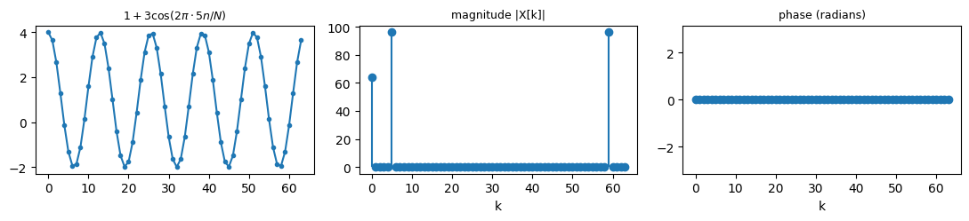
Almost every coefficient is zero. There’s a spike at $k = 0$ of height $64 = N \cdot 1$ : the constant. And there are two spikes for the cosine, at $k = 5$ and at $k = 59 = N - 5$ , each of height $96 = N \cdot 3/2$ . Why two? A real cosine is the sum of two complex exponentials rotating in opposite directions, $\cos\theta = \frac{1}{2}(e^{j\theta} + e^{-j\theta})$ , and rotating backward by 5 steps per turn looks, in sampled form, exactly like rotating forward by $N - 5$ . Each gets half the amplitude. For any real signal, the second half of the spectrum mirrors the first, $X[N-k] = \overline{X[k]}$ , so it holds no new information: to read off a real sinusoid’s amplitude, take $2|X[k]|/N$ for $0 < k < N/2$ .

Now shift the same cosine by a quarter period, $\varphi = \pi/2$ :

X = show_dft(1 + 3 * np.cos(2 * np.pi * 5 * n / N + np.pi / 2), r'$1 + 3\cos(2\pi \cdot 5n/N + \pi/2)$')
print('X[5] =', np.round(X[5], 3), '  angle:', np.round(np.angle(X[5]), 4), '  pi/2 =', np.round(np.pi / 2, 4))

X[5] = 96j   angle: 1.5708   pi/2 = 1.5708

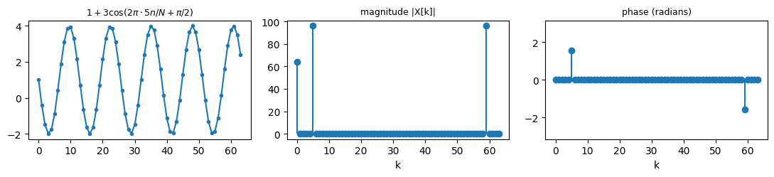
The magnitudes are identical: the signal contains exactly as much of frequency 5 as before. Only the phase changed: $X[5]$ now has angle $\pi/2$ , exactly the shift we applied (and $X[59]$ the opposite). Magnitude says what frequencies are present; phase says where their peaks and troughs fall. In fft_intro you’ll see that, for images, the phase is where most of the recognizable structure lives.

Sampling and Aliasing¶

The mirror symmetry hints at a limit. Since frequency $k$ and $N - k$ are indistinguishable in a sampled signal (as are $k$ and $k + N$ ), the highest frequency $N$ samples can represent is $k = N/2$ , one full cycle every two samples. Anything faster gets disguised as something slower. This is aliasing.

In terms of a continuous signal sampled at $f_s$ samples per second, a sinusoid of frequency $f$ can only be captured faithfully if

f_s > 2f,

the Nyquist criterion. Here’s a cosine of 7 cycles per second sampled 8 times per second, well under the required 14:

t = np.linspace(0, 1, 1000)        # "continuous" time, one second
fs = 8
ts = np.arange(fs) / fs            # 8 samples in that second

plt.figure(figsize=(8, 2.8))
plt.plot(t, np.cos(2 * np.pi * 7 * t), 'C0', lw=1, label='7 cycles/s')
plt.plot(t, np.cos(2 * np.pi * 1 * t), 'C1', lw=2, label='1 cycle/s')
plt.plot(ts, np.cos(2 * np.pi * 7 * ts), 'ko', ms=8, label='samples of the 7 cycles/s wave')
plt.xlabel('time (s)')
plt.legend(fontsize=8, loc='lower left')
plt.tight_layout()

print('samples of the 7 cycles/s wave:', np.round(np.cos(2 * np.pi * 7 * ts), 3))
print('samples of the 1 cycle/s wave: ', np.round(np.cos(2 * np.pi * 1 * ts), 3))

samples of the 7 cycles/s wave: [ 1.     0.707 -0.    -0.707 -1.    -0.707 -0.     0.707]
samples of the 1 cycle/s wave:  [ 1.     0.707  0.    -0.707 -1.    -0.707 -0.     0.707]

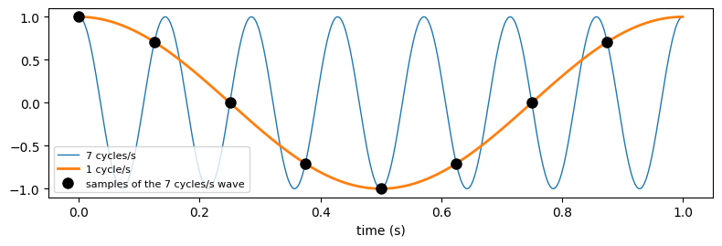
The black dots, samples of the fast blue wave, fall exactly on the slow orange one. From the samples alone there is no way to tell them apart: at 8 samples per second, 7 cycles per second is an alias of 1 cycle per second, since $7 = 8 - 1$ . Any frequency above $f_s/2$ folds back down like this.

You’ve seen this in images. When we reduced spatial resolution without anti-aliasing, fine repeating textures turned into coarse false patterns, called moiré: high spatial frequencies aliased into low ones. The cure is the one rescale(..., anti_aliasing=True) uses: blur the image before sampling, a low-pass filter that removes the frequencies above the new Nyquist limit so they can’t masquerade as lower ones.

The Fast Fourier Transform¶

Computing $X = \mathbf{F}x$ as a matrix-vector product takes $N^2$ multiplications. For a one-megapixel image, that’s far too many. The fast Fourier transform gets the identical result in about $N \log_2 N$ operations, by divide and conquer.

Split the signal into its even- and odd-numbered samples, just as the Haar step split pixel pairs. Each half is a signal of length $N/2$ with its own DFT, $E[k]$ and $O[k]$ . With a little algebra on the DFT sum, the full DFT can be assembled from them:

X[k] = E[k] + e^{-2\pi j\,k/N}\, O[k], \qquad X[k + N/2] = E[k] - e^{-2\pi j\,k/N}\, O[k], \qquad k = 0, \ldots, N/2 - 1.

Each half-size DFT can be split the same way, and so on, down to signals of length 1, whose DFT is just themselves. There are $\log_2 N$ levels of splitting, with about $N$ operations to combine at each level.

def fft_recursive(x):
    '''Radix-2 FFT. len(x) must be a power of 2.'''
    N = len(x)
    if N == 1:
        return x.astype(complex)
    E = fft_recursive(x[0::2])                        # DFT of the even samples
    O = fft_recursive(x[1::2])                        # DFT of the odd samples
    twiddle = np.exp(-2j * np.pi * np.arange(N // 2) / N) * O
    return np.concatenate([E + twiddle, E - twiddle])

x = np.random.random(1024)
print('matches np.fft.fft:', np.allclose(fft_recursive(x), np.fft.fft(x)))

matches np.fft.fft: True

Ten lines, and it agrees with NumPy. The two recursive calls handle the even and odd samples, and the last two lines apply the formula above to all $k$ at once (the factors $e^{-2\pi jk/N}$ are traditionally called twiddle factors). Let’s time the matrix product, our recursive FFT, and NumPy’s highly optimized FFT as $N$ grows.

def best_time(f, repeats=5):
    times = []
    for _ in range(repeats):
        start = time.perf_counter()
        f()
        times.append(time.perf_counter() - start)
    return min(times)

sizes = 2 ** np.arange(6, 12)    # 64 to 2048
t_matrix, t_ours, t_numpy = [], [], []
for N in sizes:
    x = np.random.random(N)
    F = dft_matrix(N)            # built outside the timing: we only time the multiply
    t_matrix.append(best_time(lambda: F @ x))
    t_ours.append(best_time(lambda: fft_recursive(x)))
    t_numpy.append(best_time(lambda: np.fft.fft(x)))

plt.figure(figsize=(6, 3.5))
plt.loglog(sizes, t_matrix, 'o-', label=r'matrix product, $O(N^2)$')
plt.loglog(sizes, t_ours, 's-', label=r'our recursive FFT, $O(N \log N)$')
plt.loglog(sizes, t_numpy, '^-', label='np.fft.fft')
plt.xlabel('N'); plt.ylabel('seconds (best of 5)')
plt.legend(fontsize=8)
plt.grid(alpha=0.3, which='both')
plt.tight_layout()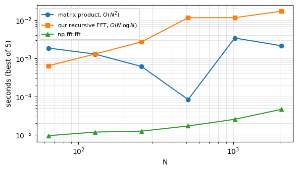

On log-log axes, the slope of each line shows how its time grows with $N$ : a slope of 2 means quadrupling with every doubling of $N$ , a slope of 1 means doubling. Your times will differ from mine, and the matrix product’s line can be bumpy, since it runs in a highly tuned linear algebra library whose speed changes abruptly once the matrix no longer fits in the processor’s cache. But the trends are clear:

np.fft.fft barely grows over this whole range, and at large $N$ it’s the fastest by far.
The matrix product is quick for small $N$ , since it’s a single call into compiled code, but it grows the fastest: over this range its time rises by a factor of hundreds or more.
Our recursive FFT is the slowest for small $N$ : it makes about $2N$ Python function calls, each with some overhead. But its line is the least steep, roughly doubling with each doubling of $N$ , so for large enough $N$ it must overtake the matrix product. (Each doubling of sizes quadruples the memory the matrix needs, which limits how far we can push the comparison.)

In the long run, the algorithm matters even more than the implementation. For a $1000 \times 1000$ image, $N = 10^6$ pixels, the difference between $N^2$ and $N \log_2 N$ is a factor of about 50,000. The FFT, popularized by Cooley and Tukey in 1965, is often called one of the most important algorithms of the twentieth century.

On to Two Dimensions¶

Like the DCT and Haar transforms, the 2D DFT is separable: transform every row, then every column of the result.

I = plt.imread('../dip_pics/moonlanding.png')
rows_then_columns = np.fft.fft(np.fft.fft(I, axis=1), axis=0)
print('separable version matches np.fft.fft2:', np.allclose(rows_then_columns, np.fft.fft2(I)))

separable version matches np.fft.fft2: True

Everything in this notebook carries over. Each 2D coefficient is the amount of one 2D wave, a stripe pattern with a frequency and an orientation, with a magnitude and a phase; real images have a mirror-symmetric spectrum; and the FFT makes it fast. That’s where Fast Fourier Analysis picks up.

🔨 Your Turn: Find the Hidden Tones¶

The cell below builds a signal from a few sinusoids, with frequencies, amplitudes, and phases chosen at random, and buries it in noise. (Don’t print the hidden values until you’ve found them yourself!)

rng = np.random.default_rng(2026)
N_hidden = 256
n_hidden = np.arange(N_hidden)
_freqs = rng.choice(np.arange(3, N_hidden // 2), size=3, replace=False)
_amps = rng.uniform(0.5, 2.0, size=3)
_phases = rng.uniform(-np.pi, np.pi, size=3)
clean = sum(a * np.cos(2 * np.pi * f * n_hidden / N_hidden + p) for f, a, p in zip(_freqs, _amps, _phases))
noisy = clean + rng.normal(0, 1.5, N_hidden)

plt.figure(figsize=(8, 2.5))
plt.plot(n_hidden, noisy, lw=0.8)
plt.title('three hidden tones, plus noise');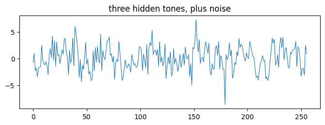

Task: Using only noisy, find the frequency, amplitude, and phase of each of the three tones. Then build a cleaned-up signal from your estimates, plot it over the noisy one, and finally compare your estimates with the hidden values (_freqs, _amps, _phases).

Guidance:

In the time domain the tones are hopeless to see. Plot the magnitude of the DFT instead. Which half of the spectrum do you need?
The noise is spread over all the frequencies, while each tone is concentrated in one. Decide what counts as a peak.
Recall from the magnitude and phase section how a cosine’s amplitude relates to $|X[k]|$ , and what the angle of $X[k]$ means.
To rebuild the signal, you can either evaluate the cosines from your estimates, or zero every DFT coefficient except the peaks (and their mirror images!) and use np.fft.ifft. Take the .real part of the result.

🧠 Further Efforts¶

Spectral leakage. Our cosines all completed a whole number of cycles in $N$ samples. Transform np.cos(2 * np.pi * 5.5 * n / N) instead, and look at the magnitude. Where did the energy go, and why? Then multiply the signal by a Hann window before transforming, and compare.
Guidance: The DFT implicitly treats the $N$ samples as one period of a repeating signal. Plot two copies of the signal end to end, and look at the seam.
Why JPEG uses the DCT, not the DFT. Take a smooth ramp, x = np.arange(64.0), and compare how much of its energy the 8 largest DFT coefficients capture (scaled with norm='ortho') versus the 8 largest DCT coefficients (make_dct_matrix(64) @ x). Explain the difference.
Guidance: The same seam as in the previous problem matters here. What does the periodic extension of a ramp look like? (The DCT corresponds to a mirrored extension.) Compare with Comparing Reconstruction Efficiency.
Convolution by multiplication. The convolution theorem says the DFT turns convolution into multiplication. Convolve a random signal with a short kernel using np.convolve, and then again by multiplying DFTs and inverting. Why don’t the results match at first, and how much zero-padding makes them match exactly?
Guidance: The DFT’s convolution is circular: what falls off one end wraps around to the other. np.fft.fft(x, n=...) pads with zeros for you.